Assessing the Impact of Terraces and Vegetation on Runoff and Sediment Routing Using the Time-Area Method in the Chinese Loess Plateau

1
State Key Laboratory of Remote Sensing Science, Faculty of Geographical Science, Beijing Normal University, Beijing 100875, China
2
College of Water Sciences, Beijing Normal University, Beijing 100875, China
3
Yellow River Conservancy Commission, Ministry of Water Resources, Zhengzhou 450003, China
*
Author to whom correspondence should be addressed.
Water 2019, 11(4), 803; https://doi.org/10.3390/w11040803
Submission received: 12 February 2019
/
Revised: 12 April 2019
/
Accepted: 13 April 2019
/
Published: 18 April 2019
(This article belongs to the Special Issue Modeling of Soil Erosion and Sediment Transport)
Abstract
:Terracing and vegetation are an effective practice for soil and water conservation on sloped terrain. They can significantly reduce the sediment yield from the surface area, as well as intercept the sediment yield from upstream. However, most hydrological models mainly simulate the effect of the terraces and vegetation on water and sediment reduction from themselves, without considering their roles in the routing process, and thus likely underestimate their runoff and sediment reduction effect. This study added the impact of terraces and vegetation practice on water and sediment routing using the time-area method. The outflow in each travel time zone was revised in each time step by extracting the watershed of the terrace units and the vegetation units and calculating the water or sediment stored by the terraces or held by the vegetation. The revised time-area method was integrated into the Land change Model-Modified Universal Soil Loss Equation (LCM-MUSLE) model. Pianguanhe Basin, in the Chinese Loess Plateau, was chosen as the study area and eight storms in the 1980s and 2010s were selected to calibrate and verify the original LCM-MUSLE model and its revised version. The results showed that the original model was not applicable in more recent years, since the surface was changed significantly as a result of revegetation and slope terracing, while the accuracy improved significantly when using the revised version. For the three events in the 2010s, the average runoff reduction rate in routing process was 51.02% for vegetation, 26.65% for terraces, and 71.86% for both terraces and vegetation. The average sediment reduction rate in routing process was 32.22% for vegetation, 24.52% for terraces, and 53.85% for both terraces and vegetation. This study provides a generalized method to quantitatively assess the impact of terraces and vegetation practice on runoff and sediment reduction at the catchment scale.
1. Introduction
Soil erosion and water loss is a serious environmental problem in the Chinese Loess Plateau [1,2,3]. It can cause soil deterioration and loss of sustainable productivity in croplands [2,4,5]. In addition, sediment yields and chemical loadings associated with soil erosion can cause severe degradation of surface water quality [6,7,8]. To control soil and water losses, terrace engineering was implemented since the 1980s and the Grain for Green (GFG) project was launched in 1999 [9,10,11,12]. Therefore, it is necessary to quantitatively analyze the effect of terraces and vegetation on runoff and sediment in the Loess Plateau.
Slope terracing and vegetation planting are common practices for soil and water conservation on sloped terrain susceptible to water erosion, and have been proven to be effective at retaining water and soil [6,13,14,15,16,17,18,19,20]. Terraces and vegetation can reduce the sediment yield from themselves significantly. Terraces reduce the peak runoff rate by reducing the slope gradient and slope length of the hillside [21,22]. Owing to the topographic slope and the embankment, terraced fields have a certain storage capacity similar to a reservoir, which can intercept surface runoff and sediment and promote runoff infiltration, evaporation, and sediment deposition [23,24,25]. The vegetation canopy can intercept rainfall directly and influence the rainfall kinetic energy and erosion rates. The stems, roots, and litter layer of vegetation can reduce runoff discharge by promoting infiltration, increasing surface roughness, and slowing down the overland flow and peak runoff. Vegetation also can reduce soil erosion by reducing surface flow volume and increasing sediment trapping through reducing flow velocity [21,26,27]. In addition to this, both terraces and vegetation can intercept the sediment yield from upstream and achieve sediment reduction in the valley by reducing runoff flowing from the slope into the valley [16,24,28,29].
Numerous studies have provided many insights into how terraces and vegetation control water erosion at local scales using observational experiments [20,27]. Terraces could be classified into level terraces, slope terraces, slope-separated terraces, and zig terraces according to their structure [23]. In the Loess Plateau of China, the main terrace type is level terraces. Yao [30] found a terraced field could reduce soil erosion by 92–100% compared with sloped farmland, while Wu [31] found the average benefit of level terraces on soil and water conservation were 86.7% and 87.7%, respectively. Huo and Zhu [32] combined soil water moisture and 137Cs content analysis and found the average soil and water conservation benefit of level terraces was 53%_ENREF_18, while Pan and Shangguan [27] reported that grassplots had 14–25% less runoff and 81–95% less sediment yield compared to a bare soil plot. Meng et al. [33] conducted a series of laboratory flume simulation experiments and the results showed that vegetation could reduce the mean velocity by 31–65%_ENREF_36. As the effectiveness of terraces and vegetation is limited by many factors, such as climate, soil properties, topography, land use, vegetation type, and spatial patterns, the diversity and natural variability of previously conducted erosion studies limit their potential extrapolation to the catchment scale [23,34,35,36]. Thus, how to assess the effects of terraces and vegetation on water erosion control at the catchment scale remains a crucial issue.
Estimation of rainstorm-generated sediment yield by means of a hydrological model is an important way to quantitatively evaluate the effect of soil and water conservation measures, such as by using the Soil and Water Assessment Tool (SWAT) model [37,38,39], the Agricultural Non-Point Source pollution (AGNPs) model [40], and the Agricultural Policy/ Environmental eXtender (APEX) model [41]. In these models, accounting for the impact of terraces and vegetation on runoff and sediment yields has focused on reduction from themselves through adjusting the key input variables, such as the Soil Conservation Service Curve Number (SCS-CN), slope gradient, slope length, Universal Soil Loss Equation (USLE) support practice factor (P-factor), and cover and management factor (C-factor) [11,21,22,25,29,42,43], without considering the roles of water and sediment reduction in the routing process. Then, the runoff and sediment reduction effect of terraces and vegetation is likely to have been underestimated. Therefore, it is necessary to take into account the water and sediment reduction effect of terraces and vegetation in the model’s routing process.
Explicitly simulating the interaction between conservation practice and watershed response is difficult. The time-area method, with its inherently distributed concept, explains which parts of a watershed contribute to runoff during a specific period [44]. It provides a simple and useful tool to understand runoff mechanisms and is widely used at the catchment scale [44]. It has also been indicated that the routing of sediment through time-area segments in a catchment produces better results than the conventional routing through a network of cells [45,46]. Her and Heatwole [47] revised the time-area method and considered the upstream contribution for routing sediment, such that the new method provided detailed spatial representation_ENREF_15. These studies mainly focused on the effect of surface heterogeneity on routing time or flow velocity [48,49]. Topographic features are delineated through a Digital Elevation Model (DEM), slope gradient, flow direction, and so on. However, the lack of representation of a specific terrace and vegetation process makes it difficult to quantitatively distinguish vegetation and terraced fields and their integrated ability for water and sediment reduction.
Thus, the purpose of this study was to incorporate the effect of terraces and vegetation on runoff and sediment routing in the time-area method and assess their impact in water and sediment reduction. The outflow in each travel time zone was revised in each time step by extracting the watershed of the terrace units and the vegetation units, and calculating the water or sediment stored by the terraces or retained by the vegetation based on their properties.
2. Materials and Methods
2.1. Study Area
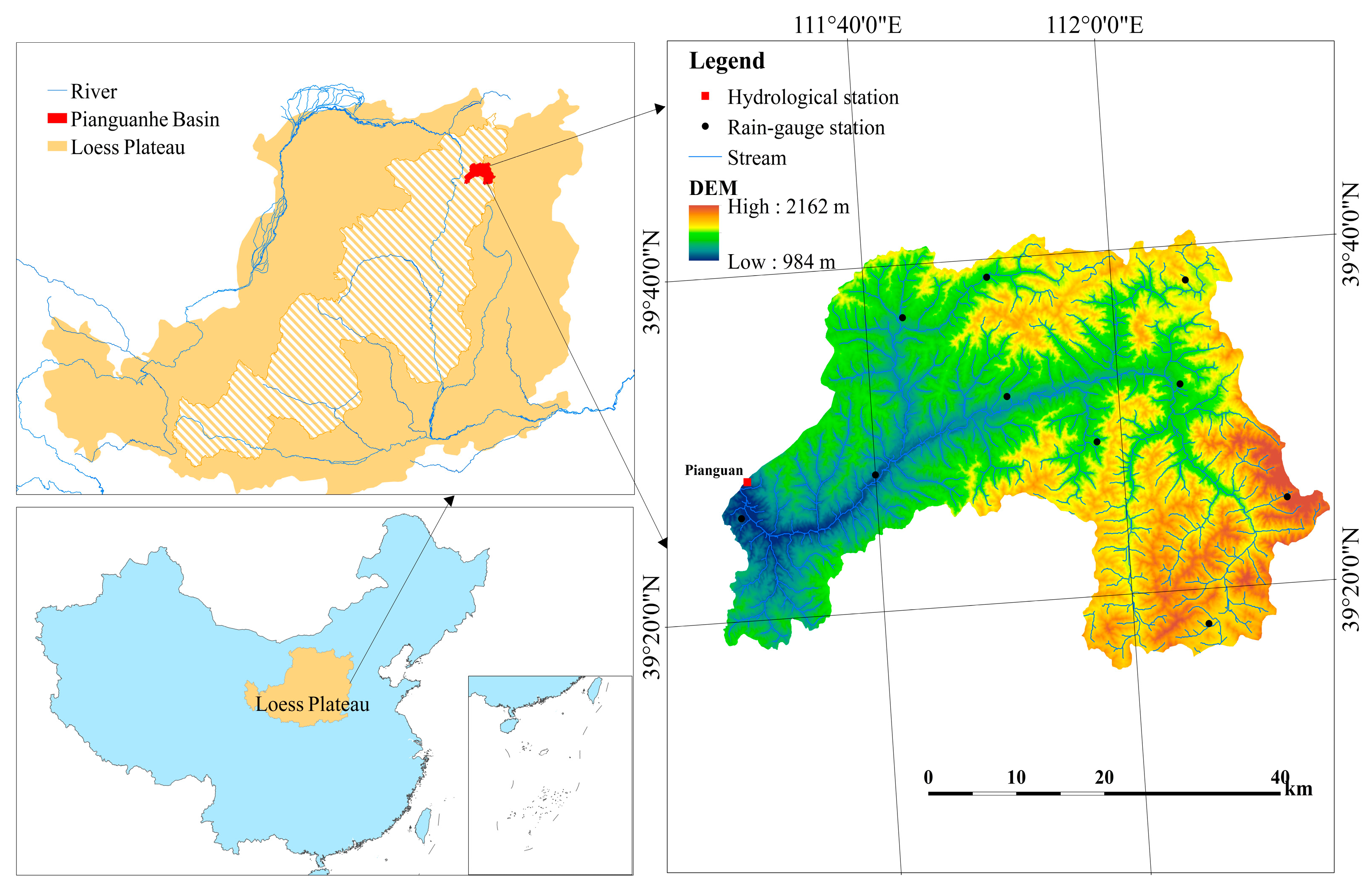
In this study, we selected the Pianguanhe River in the key soil erosion region of the Loess Plateau as our case study. The Pianguanhe River is located in the hilly and gully region of the Loess Plateau (111°26′ E–112°17′ E, 39°15′ N–39°42′ N) (Figure 1). It is a tributary of the Yellow River with a watershed area of 2089 km2, with altitude ranging from 984 to 2162 m. The study area features a semi-arid continental climate, with an average annual rainfall of 429 mm. The uneven seasonal distribution of precipitation results in more than 80.9% of the annual precipitation occurring from May to September [50]. The average annual runoff and sediment discharge is 39.48 million m3 and 12.58 million t, respectively. The sediment modulus is 65.23 t/ha/yr [50]. The overall loss of soil and water is a serious environmental issue.
2.2. Methods
The serious soil and water loss in the Loess Plateau has always occurred because of the surface runoff caused by heavy rains. In this paper, runoff generation was simulated based on the Land Catchment Model (LCM), which is a flood event forecasting model that was developed through more than 300 artificial rainfall experiments in the Loess Plateau [51,52]. The model has been modified into a distributed model [53,54,55]. The Modified Universal Soil Loss Equation (MUSLE) was chosen to estimate the sediment yield of individual heavy rainfall events [56], and numerous studies had proven its applicability to estimate the sediment yield in the Loess Plateau [57,58,59]. The main functions of LCM-MUSLE model are listed in Table 1 and Table 2. The reader is referred to Luo et al. [59] for a detailed description of the LCM-MUSLE model, which is not described here. Runoff and sediment generation from sub-catchments was routed to the outlet by considering overland flow and stream channels. Time-area method was used for overland routing [49] and Muskingum method was used for channel routing [60,61].
With the purpose of simulating the influence of terrace and vegetation units on water and sediment reduction at confluences, as the critical hydrologic process, both terrace and vegetation modules were added to the time-area method. In the time-area method, the catchment is divided into a number of travel time zones via isochrones [67]. By extracting the watershed of terrace units and vegetation units, and calculating the water stored by the terraces or intercepted by vegetation, the runoff yield and the outflow in each travel time zone are revised. This represents the spatiotemporally varied flow in the routing simulation. Sediment reduction was achieved in a similar way.
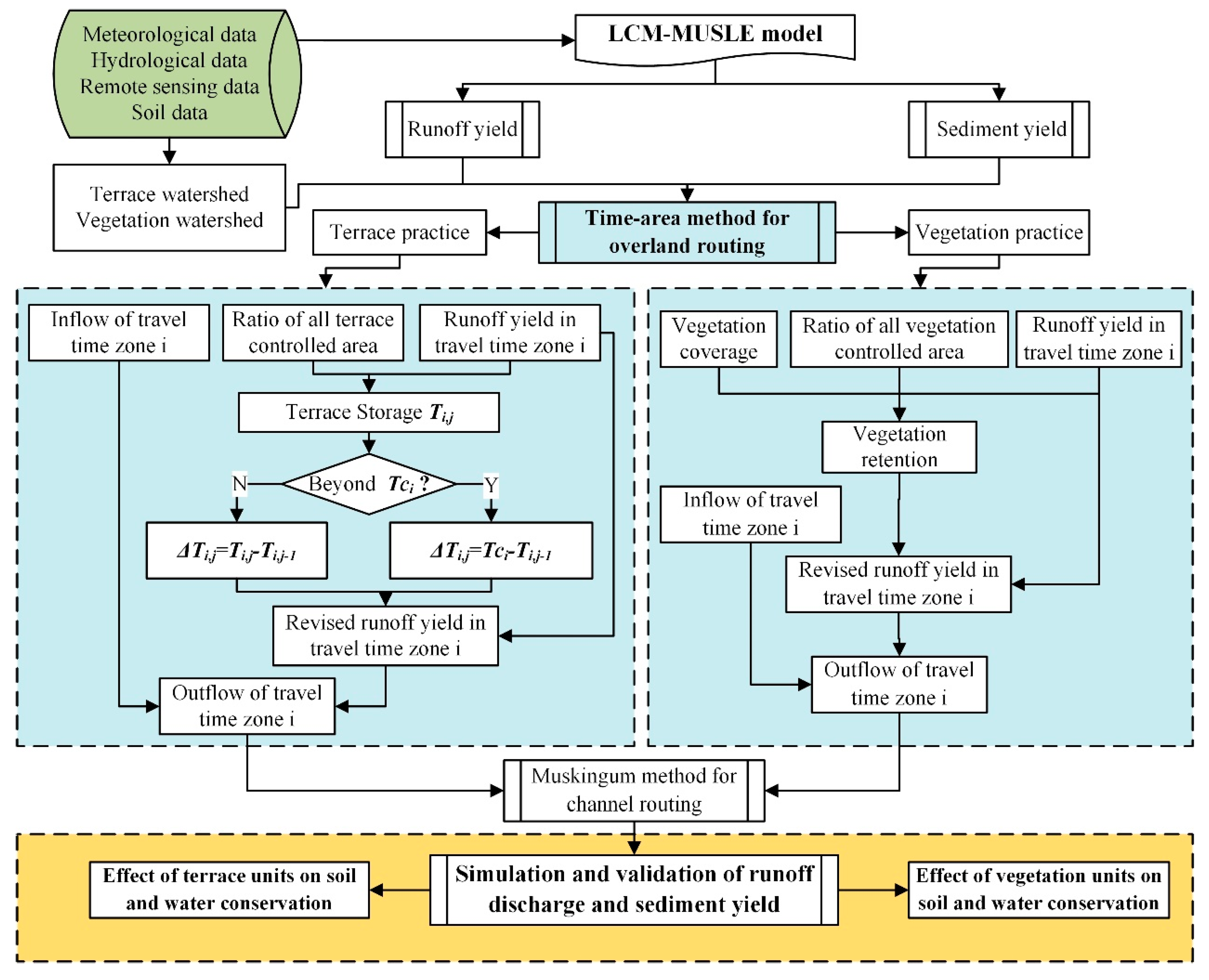
The integrated structure of the model is shown in Figure 2. Specific equations and methods are discussed in the following sections. The integrated model can represent landscape heterogeneity in detail, if a higher spatial resolution DEM is used.
2.2.1. Time-Area Method for Overland Routing
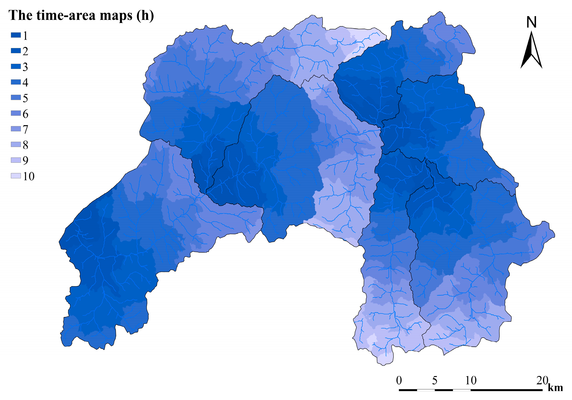
Isochrones are defined as the contours of equal travel time to the catchment outlet, and the travel time zone is the area between two adjacent isochrones [67]. The isochrones of the whole basin are calculated, and then these are adjusted within each sub-catchment, as shown in Figure 3. It is assumed that the area of each time zone is ΔA1, ΔA2, ···, ΔAn, and their corresponding travel time is τ1, τ2, ···, τn, respectively. Then, we set Δτ = τi − τi−1 (i = 1, 2, ···, n). It is assumed that m is the time of runoff generation in hours, ΔRr (r = 1, 2, …, m) is the runoff depth in m, and the runoff discharge of the outlet at time step j is:
For n ≥ m
If j < m, k = j; if j ≥ m, k = m, and if j > n, ΔA = 0.
For n < m:
If j < n, k = j; if j ≥ n, k = n, and if j > m, ΔR = 0.
For travel time zone i, its runoff discharge at time step j can be calculated as follows:
where Qi,j is the outflow from travel time zone i at time step j (m3); and Qi+1,j−1 is the outflow from time zone i + 1 at time step j − 1 (m3).
Unlike runoff routing, sediment transport simulation gave consideration to the sediment particle size and the hydraulic characteristic of the basin. It was calculated using Equation (4), as suggested by Williams [68]:
where RY is the sediment yield for the entire basin (t); Yi is the sediment yield for the sub-catchment i before routing to channel (t); B is the routing coefficient; Ti is the travel time from the sub-catchment i to the basin outlet (h); and D50i is median particle diameter of the sediment for sub-catchment i (mm).
2.2.2. Extraction of the Terrace Units and Vegetation Units Watershed
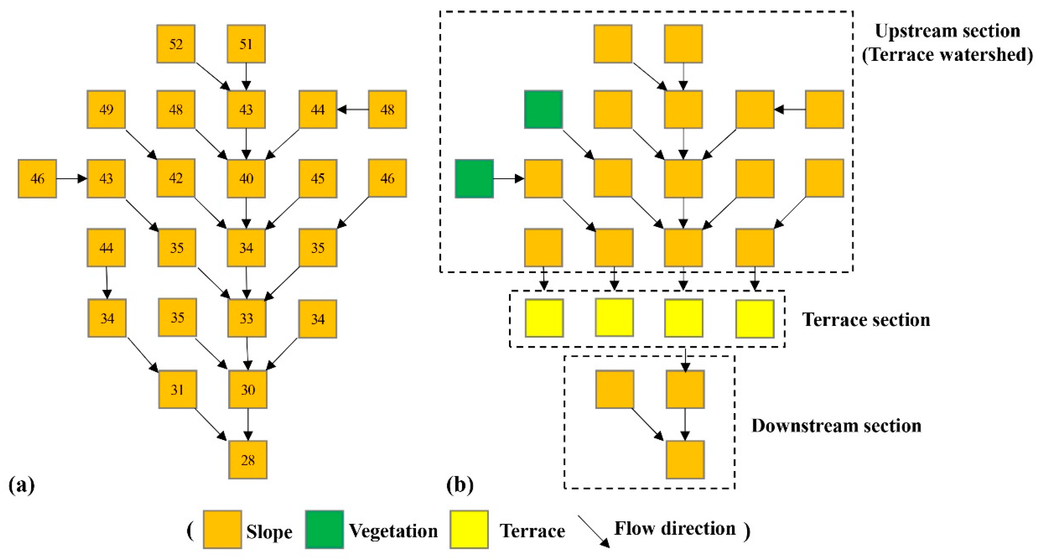
The impact of terrace and vegetation units on water and sediment flow depends upon their size and position in the catchment. The flow direction of the natural hillslope is shown in Figure 4a. When there is a terrace in the hillslope, the connectivity of its original flow pathways is broken, and the whole slope could be divided into three segments: upstream section, terrace section, and downstream section (Figure 4b). Here, we define the upstream section as the watershed of terrace (or runoff contributing area). The area impacted by the terrace units in terms of water and sediment reduction is the total of the terrace and its watershed.
The terrace watershed was extracted by searching upward from the terrace cell based on deterministic-8 (D8) flow direction method [69]. For each cell, once there was a route that water could follow to reach the terrace cells, the cell was considered to belong to the terrace watershed. The extraction of vegetation watershed was the same as that for the terrace watershed.
2.2.3. Consideration of Terrace Units in the Time-Area Method
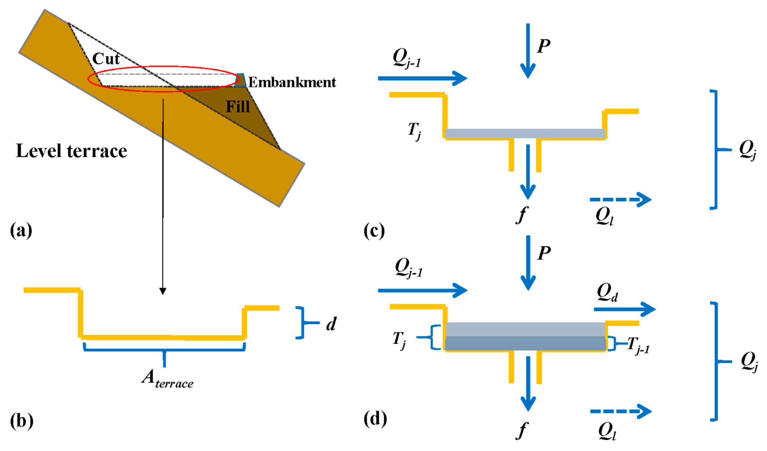
The revised time-area method simplifies a level terrace as a dynamic water tank, and its storage capacity is the product of the terrace area and the embankment height (Figure 5a,b). In this study, we made the assumption that the stream flow in a terrace should only be considered as the overflow, regardless of the drainage discharge. Namely, when the water trapped by the terrace exceeds the terrace storage capacity during heavy rainfall events, the surplus water will overflow (Figure 5c,d).
Referring to Equation (3), when there are terrace units occurring in time zone i, the outflow Qi,j from time zone i at time step j is revised, as follows:
where Qi+1,j−1 is the outflow from time zone i + 1 at time step j − 1 (m3); ΔTi,j is the increased water ponded in terraces that are located in time zone i at time step j (m3). When ΔTi,j equals 0, the storage capacity of the terraces is filling up and they can no longer have a retention function.
Before filling up, the current terrace storage volume is the sum of its previous storage volume and the current terrace watershed inflows. Due to the possible distribution of several terraces in a time zone and due to the fact that each terrace may correspond to multiple cells, the statistics of the water interception of each terrace requires a large amount of calculations. In order to simplify the complex problem, we estimated the terrace watershed inflows as a percentage of the runoff generation in the time zone, and the percentage equals the area ratio of all terraces control area to the time zone. Then ΔTi,j is calculated as follows:
where Ti,j is the amount of stored water in all terraces in time zone i at present time step j (m3); Ti,j−1 is the amount of stored water in all terraces in time zone i at previous time step j − 1 (m3); Tci is the maximum water storage of all terraces in the time zone i (m3); Tui is the ratio of all terrace control area in the time zone i; ΔATcontrol,i is the area of all terrace control area in time zone i (m2); ΔAterrace,i is the total area of terraces in time zone i (m2); and di is embankment height of terrace (m). As runoff is the main carrier of sediment, the increased sediment stored by terraces in time zone i at time step j equals the sediment yield in time zone i at time step j multiplied by the runoff trapped rate of terraces in time zone i at time step j (namely, the ratio of ΔTi,j to ΔRjΔAi).
Taking Equation (6) and Equation (7) into Equation (5), we can get the outflow Qi,j as follows:
2.2.4. Consideration of Vegetation Units in the Time-area Method
Unlike terraces, which can act as a water tank, vegetation does not have a direct storage volume, but it can resist the confluence process of runoff and sediment. Vegetation coverage and canopy density are the main indicators influencing vegetation’s impact on water and soil conservation [70,71,72]. In this study, we chose vegetation cover that was easily derived to incorporate the vegetation module into the time-area method.
Similar to Equation (5), when there are vegetation units occurring in time zone i, the outflow Qi,j from time zone i at time step j is as follows:
where ΔVegi,j is the water or sediment trapped by vegetation units in time zone i at time step j (m3).
ΔVegi,j is calculated as follows:
where Vui is the ratio of all the vegetation control area in the time zone i; ΔAVcontrol,i is the total area of vegetation in time zone i (m2); Veg is vegetation coverage (%); is function of Veg, it refers to runoff or sediment retention rate of the forestland or grassland with certain vegetation coverage, and is the average value of runoff or sediment retention rates in the time zone i.
Most flume test researches in the Loess Plateau lack the complete information about the runoff and sediment retention rate of grassland and forestland with different cover [73,74,75,76]. Xiong et al. [77] systematically deconstructed the experimental data from different slope runoff plots in the Loess Plateau, and summarized benefit indices of runoff and sediment reduction by forestland and grassland of different qualities in years with different runoff and sediment levels [77], as shown in Table 3. This paper refers to the study of Xiong et al. [77]. For the convenience of distributed calculation, we fitted the data in Table 3 to get the runoff and sediment reduction functions of forestland and grassland under different conditions, as shown in Table 4 and Table 5, x means vegetation coverage (%) and y means runoff and sediment reduction rates.
2.2.5. Model Performance Evaluation Criteria
Nash–Sutcliffe efficiency (NSE) was used to evaluate the performance of the simulation:
where Oi is observed data (runoff discharge or sediment discharge); Ei is simulated data (runoff discharge or sediment discharge); is average observed data; N is number of values. NSE varies from negative infinity to 1, where NSE closer to 1 indicates a better simulation.
A total of eight isolated storms with observed runoff and sediment yield were selected to calibrate and verify the model. There were five in the 1980s, and three in the 2010s, and each storm was encoded with its start time as Nos. year/day/hour. Among them, Nos. 1981/203/17, 1983/215/22 and 1983/235/16 were used for calibration, while Nos. 1988/199/13, 1989/203/19, 2006/195/5, 2006/224/8 and 2010/263/20 were used for validation.
The runoff and sediment simulation was implemented in four cases: O1—original simulation without considering terrace and vegetation practice; R1—revised with vegetation module; R2—revised with terrace module; R3—revised with vegetation and terrace modules. For the five events in the 1980s, as the terrace data was unavailable and terraces just accounted for a small proportion of the area, only O1 and R1 were simulated. For three events in the 2010s, all four cases were simulated. The terraces in the study area are all level terraces with good quality [78], and we made an assumption that all terraces had an embankment height of 20 cm. For vegetation, the retention functions of runoff and sediment were chosen according to the rainfall amount of each event and the rainfall condition of the two days before each event. Here, for Nos. 1983/215/22, 1983/235/16, 1988/199/13, 2006/224/8 and 2010/263/20 functions of normal period were chosen in Table 4 and Table 5, while for Nos. 1981/203/17, 1989/203/19 and 2006/195/5 functions of wet period were chosen.
2.3. Data Source
Input data for the model included hourly precipitation, DEM, land use, vegetation coverage, soil data, and particle size of the sediment. In addition, observed runoff and sediment discharge of hydrological stations were used in the model’s calibration and validation.
- (1)
- Hourly precipitation was collected from 10 rain-gauge stations (Figure 1). The gauge data were interpolated by the inverse distance weighted (IDW) method to acquire the spatial data.
- (2)
- Advanced Spaceborne Thermal Emission and Reflection Radiometer Global Digital Elevation Model (ASTER GDEM) was selected to extract topographical information, river network, sub-basins and isochrones (http://www.gscloud.cn/).
- (3)
- Land use and vegetation coverage were derived from Landsat images (http://www.gscloud.cn/). Land use was classified into 11 types, including cropland (slope < 6°), cropland (6° < slope < 25°), cropland (slope ≥ 25°), forest, shrub, open woodland, immature forest land and orchard, grassland, water area, developed land, and other land. Vegetation coverage was derived based on its relation with normalized difference vegetation index (NDVI) [79], while the vegetation coverage of cropland was not included in routing process. Land use and vegetation coverage data from 1978 and 2010 were used to represent data for 1980s and 2010s, respectively.
- (4)
- Terrace data in 2012 was acquired from the Yellow River Conservancy Commission (YRCC), which was interpreted from ZY-3 images with a spatial resolution of 2.5 m and an accuracy of 94% [78].
- (5)
- The soil types, sand content, silt content, clay content, organic carbon, and gravel content were derived from the Harmonized World Soil Database (HWSD), and the soil saturated moisture of each soil type were determined from the software Soil-Plant-Atmosphere-Water Field & Pond Hydrology (SPAW).
- (6)
- The measured discharge, sediment concentration and median of sediment particle size (D50) at the Pianguanhe hydrological station were acquired from the YRCC.
All data were reproduced at 30 × 30 m spatial resolution and projected to Albers, using the World Geodetic System-84 (WGS84) datum. Data were processed by ENVI5.1 (Harris Corporation, Melbourne, FL, USA), GisNet [80], ArcGIS10.4.1 (Environmental Systems Research Institute, Redlands, CA, USA), or programs written in IDL (Interactive Data Language).
3. Results
3.1. Watershed of Terrace Unit and Vegetation Unit
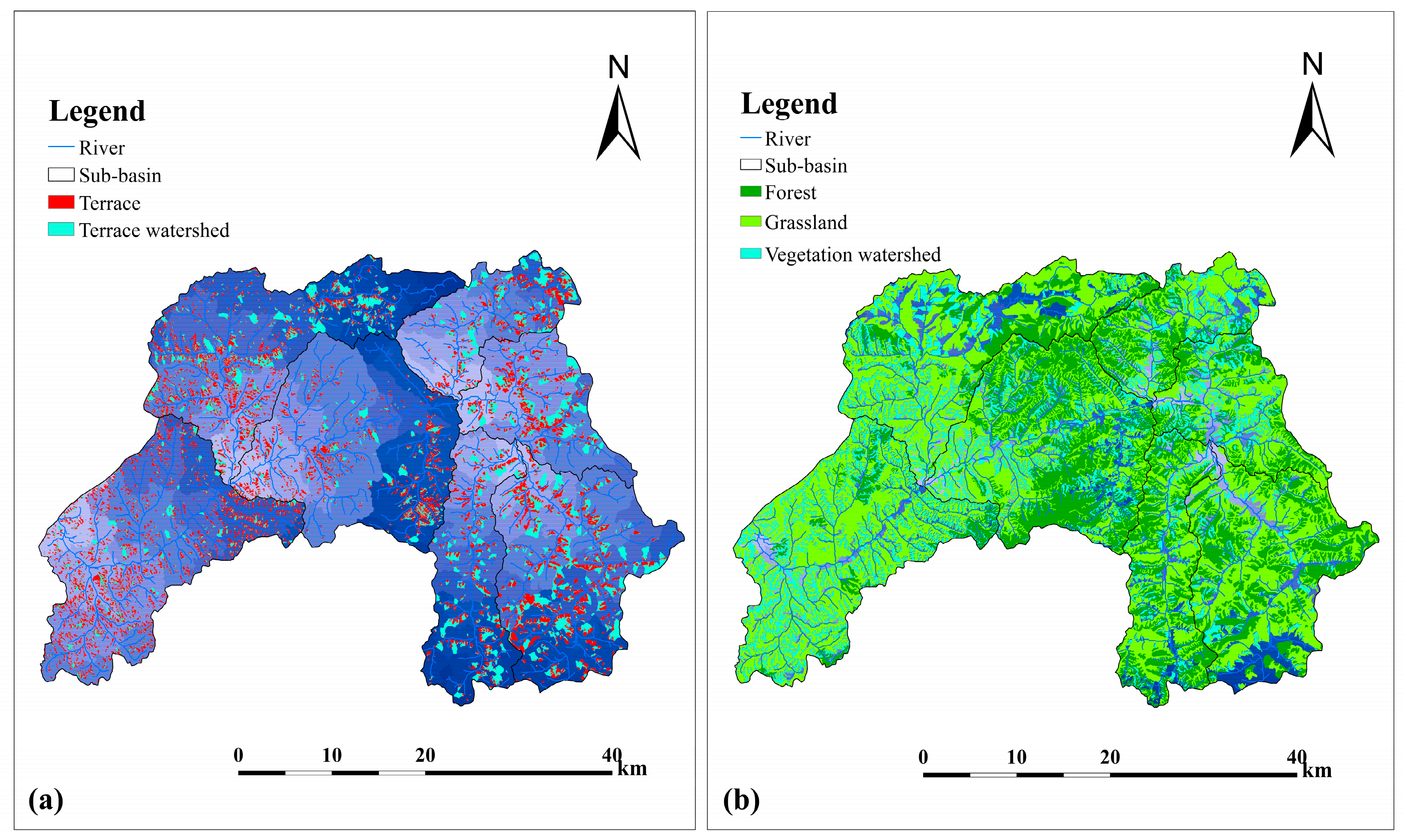
The terrace ratio is the proportion of terrace area to water and soil loss area [78]. In 2012, the total terrace area of Pianguanhe was 189.32 km2, accounting for 9.87% of the whole basin and giving a terrace ratio of 10.18%. The terrace ratio of Pianguanhe was 1.80% in 1979 [50]. In view of data availability, we chose terrace data from 2012 (to represent the 2010s) and extracted its terrace watershed. The terrace watershed was 169.90 km2 in 2012. The terrace control area is the sum of terrace area and terrace watershed and accounted for 1.89 times the area of the terrace, as shown in Figure 6a.
The area of forestland and grassland in Pianguanhe was 1328.70 km2 in 1980s and 1349.17 km2 in the 2010s, giving an increase of 20.47 km2. The average vegetation coverage was 22.27% in 1980s and 62.74% in the 2010s, giving an increase of 40.47%. Thus, the vegetation quality demonstrated a significant increase compared to the area. We extracted the vegetation watersheds in the 1980s and 2010s. Figure 6b shows the vegetation watershed of Pianguanhe in the 2010s. Vegetation control area was the sum of vegetation units and vegetation watershed. It was 1675.77 km2 in the 1980s and 1693.96 km2 in the 2010s, indicating that it did not change very much.
3.2. Validation of Runoff Discharge
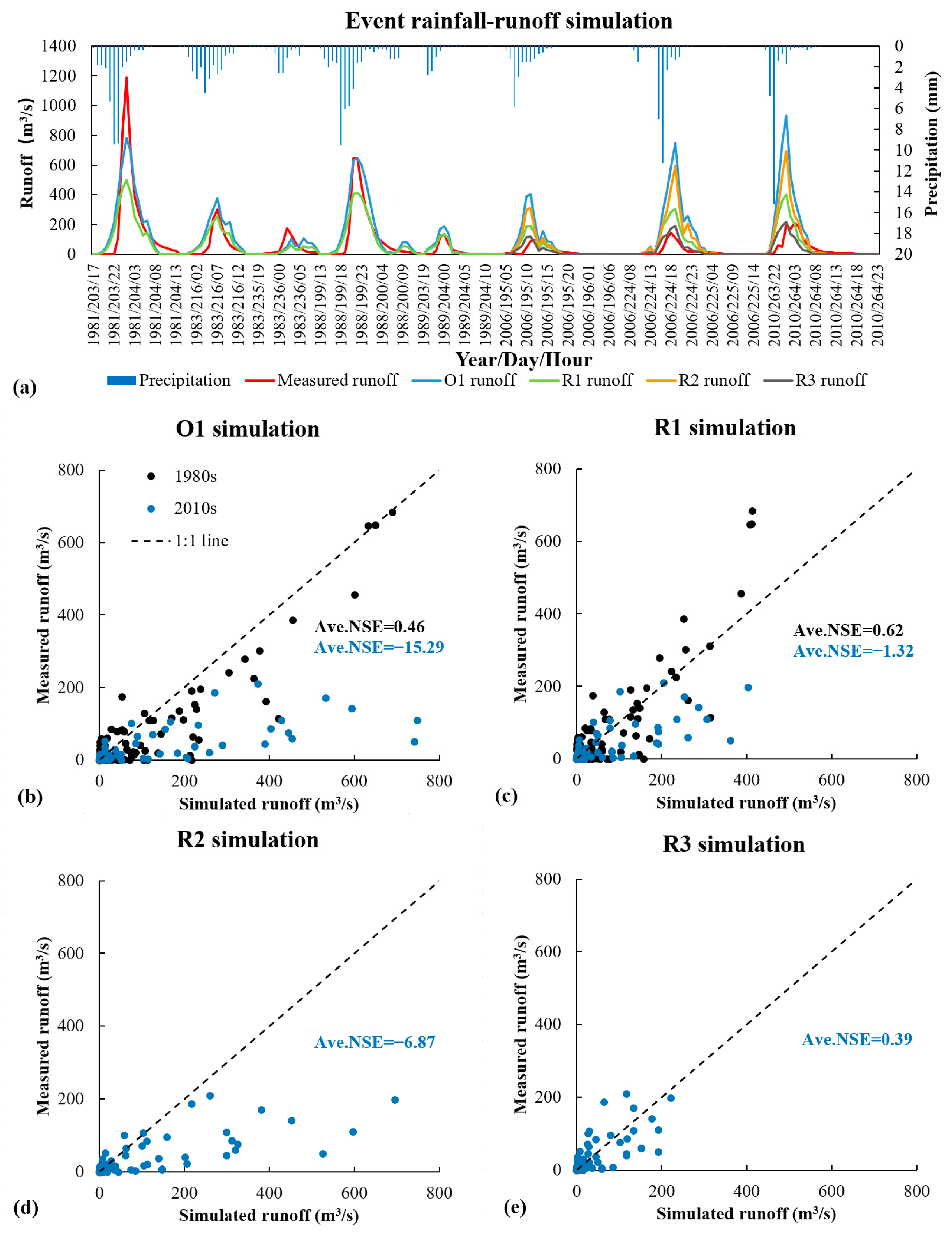
Figure 7a presents the event-based comparison between the measured runoff discharge and the runoff discharge predicted under different cases. The simulated runoff discharge in most events were comparable to their measured values. For the five events in the 1980s, the peak values of R1 were lower than those of O1. For the three events in the 2010s, the peak values rank from lowest to highest: R3 < R1 < R2 < O1 (Figure 7a). This shows that the revised simulation with vegetation can significantly reduce the runoff peak compared to the simulation with terrace, and that the simulation considering both terrace and vegetation was closest to the estimated value.
Comparison of the simulated runoff with the measured runoff is shown in Figure 7b–e. Figure 7b shows the validation of O1, in which the five events in the 1980s achieved an average NSE of 0.46, while the three events in the 2010s achieved an average NSE of −15.29. The data points of the 1980s are distributed close to the 1:1 line, while the data points of the 2010s are distributed farther away from the 1:1 line. It shows that the original model did not achieve good performance for recent years, since the surface had undergone significant change. Figure 7c shows that the average NSE of the 1980s and 2010s both increased in R1, with the average NSE of the 2010s showing a greater increase (value of −1.32), and the data points of the 2010s distributed closer to the 1:1 line than in the O1 validation shown in Figure 7b. Figure 7d shows the R2 validation, and indicates that the average NSE of the 2010s has also increased compared with that of O1, but that the extent of the increase is less than for R1. Figure 7e shows the R3 validation and indicates that the average NSE of the 2010s is 0.39, which for the first time is positive, and that the data points of the 2010s are closely distributed around the 1:1 line. Overall, the simulation accuracy of the 2010s is highest in R3, followed by R1. These figures show that the revised model was better at simulating the runoff in recent years and can reflect the effect of significant surface change (i.e., slope terracing and revegetation) on runoff.
3.3. Validation of Sediment Discharge
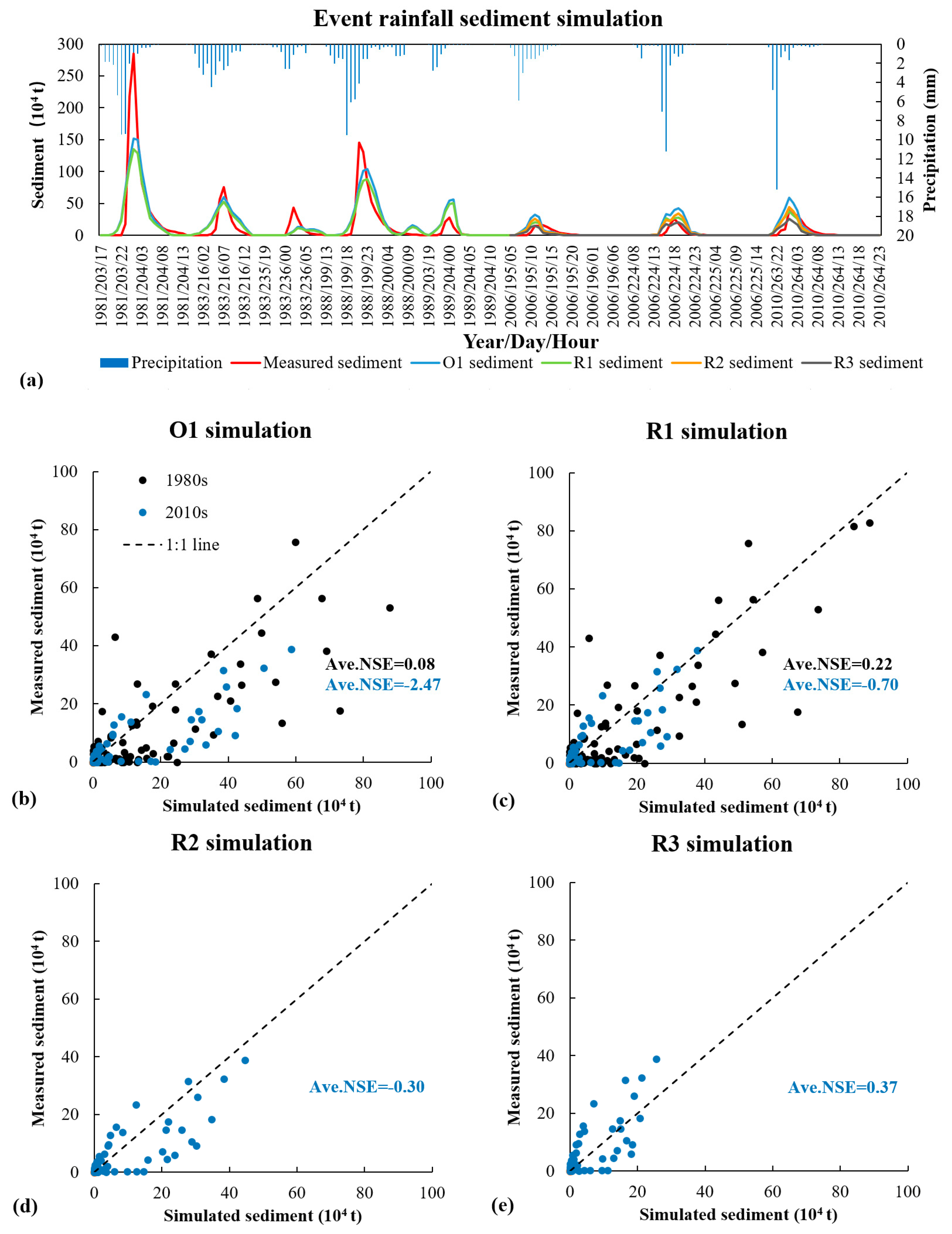
The hourly measured sediment concentration (kg/m3) along with the measured runoff discharge were converted to get sediment discharge (t/h). Figure 8a shows the event-based comparison between the measured and predicted sediment discharge under different cases. The simulations of sediment discharge were in good agreement with their measured values in most events. The difference between the sediment discharge of O1 and measured values is smaller than the runoff discharge between O1 and measured values in recent years; it was because the sediment reduction was partly achieved in the sediment yield process through the C and P factors in MUSLE. For the five events in the 1980s, the peak values of R1 were lower than those of O1. For the three events in the 2010s, the peak values rank from lowest to highest were: R3 < R1 < R2 < O1 (Figure 8a). This shows that the revised simulation with vegetation can significantly reduce the sediment peak compared to the simulation with terrace, and that the simulation considering both terrace and vegetation was closest to the estimated value.
NSE was also used to evaluate the performance of the simulated sediment discharge, as shown in Figure 8b–e. Figure 8b shows the O1 validation, in which the five events in the 1980s achieved an average NSE of 0.08, while the three events in the 2010s achieved an average NSE of −2.47. It shows that the original model did not achieve good performance in the recent years. Figure 8c shows the R1 validation, in which the average NSE of the 1980s and 2010s both increased. The data points of the 1980s and 2010s were distributed closer to the 1:1 line than in Figure 8b. Figure 8d shows the R2 validation, in which the average NSE of the 2010s have also increased, and greater than that of R1, which indicates that terrace can significantly reduce sediment. Figure 8e shows the R3 validation, in which the average NSE of the 2010s is 0.37, and the data points of the 2010s are distributed closely around the 1:1 line. Overall, the accuracy of the simulation in the 2010s is highest in R3, followed by R2. These figures show that the revised model performs better in recent years, and can reflect the effect of significant surface change (i.e., slope terracing and revegetation) on sediment yield.
4. Discussion
4.1. Effect of Terraces and Vegetation on Runoff Reduction
To quantify the reduction effects of vegetation and terracing during runoff and sediment routing process, the absolute reduction in unit area (AR) and the reduction rate (RR) were calculated. In the case of runoff, for example, we first summed the hourly runoff discharge to obtain the total runoff of each rainfall, and counted the total simulated runoff of each event per case. We then calculated the AR of R1 and R2, and the RR of R1, R2, and R3, as shown in Table 6. The AR and RR were calculated as follows:
where y is total simulated runoff of O1 (m3); and yi is total simulated runoff of R1, R2 or R3 (m3), Ai is total area of R1 or R2 (km2).
As shown in Table 6, the average RR of R1 on runoff was 33.58% in the 1980s. For the three events in the 2010s, the average RR of R1 was 51.02%, the average RR of R2 was 26.65%, and the average RR of R3 was 71.86%. The average AR of R1 was 3051.42 m3/km2 per event, and it was 15809.18 m3/km2 for R2. The results show that the runoff reduction rate of vegetation was significantly higher than that of terraces, as the area of vegetation is seven times larger than that of terraces. However, terraces could reduce more runoff per unit area. Influenced by the revegetation and increase in vegetation coverage, the average RR of R1 in recent years increased by 17.44% over that in the 1980s. In general, the effectiveness of runoff reduction was highest under R3. Besides, the sum of RR1 and RR2 is inconsistent with RR3. The reason for the latter might be that when the terraces had played the role of water reduction, the water reducing capability of vegetation in the same time zone would be decreased. The assumption that all terraces in the Pianguanhe Basin are of good quality and have the same embankment height may be an oversimplification that overestimated the runoff reduction efficiency of the terraces.
4.2. Effect of Terraces and Vegetation on Sediment Reduction
We counted the total simulated sediment yield of each event per case, and also calculated the AR of vegetation and terraces, and the RR of R1, R2, and R3, as shown in Table 7. The average RR of R1 for sediment was 13.31% in the 1980s. For the three events in the 2010s, the average RR of R1 was 32.22%, the average RR of R2 was 24.52%, and the average RR of R3 was 53.85%. The average RR of R1 in recent years increased by 18.91% over that in the 1980s. The average AR of R1 was 449.95 t/km2, and 2850.17 t/km2 for R2. The results also show that the sediment reduction rate of vegetation was higher than that of terraces, but that terraces could reduce more sediment per unit area. In general, the effectiveness of sediment reduction of R3 was highest. Besides, the sum of RR1 and RR2 was inconsistent with RR3. As mentioned previously, the reason might be that when terraces had played the role of sediment reduction, the sediment reducing efficiency of vegetation in the same time zone would be decreased. The assumption that all terraces in the Pianguanhe Basin are of good quality and have the same embankment height may have overestimated the sediment reduction efficiency of terraces.
4.3. Reliability Analysis of the Water and Sediment Reduction Efficiency of Terraces and Vegetation
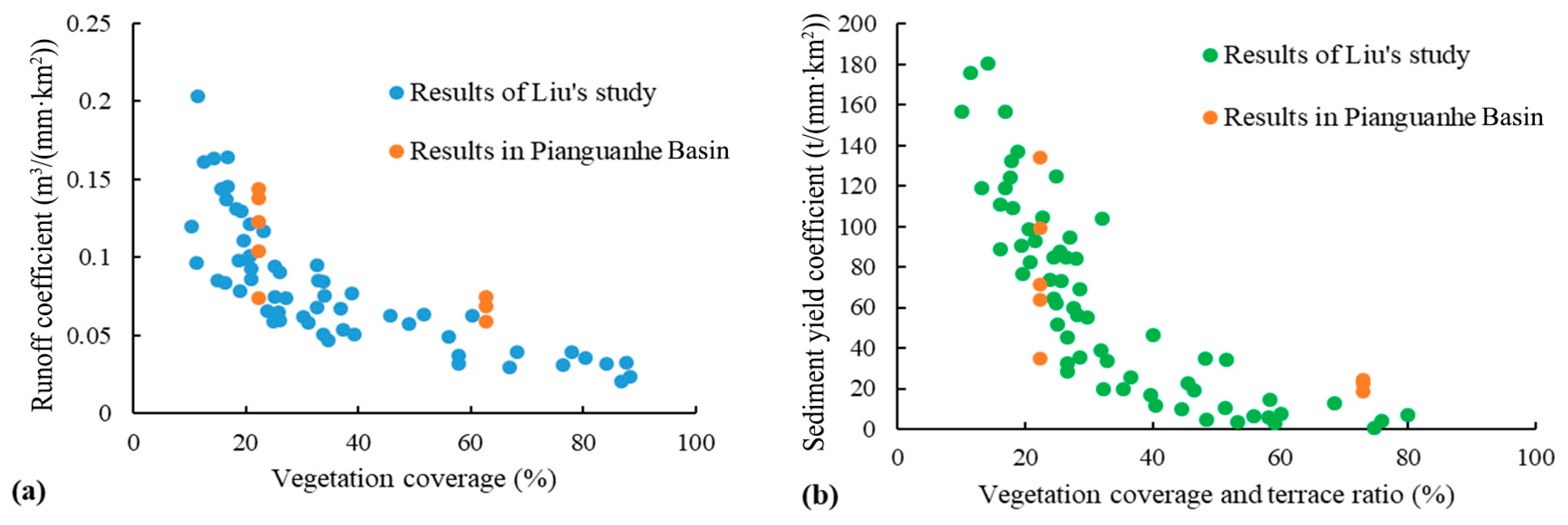
Liu et al. [78,81] introduced a runoff coefficient and sediment yield coefficient to discuss the flood and sediment yield for different vegetation conditions at the catchment scale in the Loess Plateau. To analyze the reliability of the simulation results, we also calculated the runoff coefficient and sediment yield coefficient of each event in the Pianguanhe Basin, and compared with the results of Liu et al. [78], as shown in Figure 9a,b. The runoff coefficient is the runoff yield per unit of precipitation per unit area, while the sediment yield coefficient is the sediment yield per unit of precipitation per unit area. In Liu et al. [78], the runoff coefficient was calculated based on annual runoff and precipitation data, and the latter only considered rainfall greater than 25 mm. In this study, the runoff coefficient was calculated based solely on storm event discharge and rainfall data. Thus, there is a disparity between the calculation results of these two studies, but yet the results are comparable to those of Liu et al. [78]. The runoff coefficient decreased along with the increase of the vegetation coverage. The vegetation coverage of the 1980s and 2010s was 16.17% and 46.29%, respectively, and the average runoff coefficient decreased from 0.12 m3/(mm·km2) in the 1980s to 0.07 m3/(mm·km2) in recent years.
Similarly, the sediment yield coefficients calculated from the event data in this study are different from those of Liu’s results based on calculations using annual data, and yet the results are comparable. The sediment yield coefficients also decreased along with the increase of vegetation coverage. The average sediment yield coefficient decreased from 80.68 t/(mm·km2) in the 1980s to 21.93 t/(mm·km2) in recent years.
4.4. Limitations and Potential Improvements
While this study assessed the impact of terraces and vegetation practice on runoff and sediment routing process using the revised time-area method, it still has several assumptions and limitations in the method that need to be clarified and studied further. First, embankment height is a key indicator to evaluate the quality and storage volume of terraces. The assumption that all terraces in the Pianguanhe Basin are of good quality and set the embankment height with a fixed value may overestimate the runoff and sediment reduction efficiency of the terraces. This paper referred to the study of Xiong et al. [77] as the limitation of the flume test data. While the runoff and sediment retention function of vegetation is not independent of slope steepness or vegetation structure, these factors have not been considered yet. In addition, the effect of engineering measures such as check dam and human factors such as mining and road construction should also be considered to further improve simulation efficiency.
5. Conclusions
In this study, we added the impact of terrace and vegetation practice on runoff and sediment routing in the time-area method. The revised time-area method was integrated into the LCM-MUSLE model which is suitable to estimate the water and sediment yield in the Loess Plateau. Eight isolated storm events in the 1980s and 2010s in Pianguanhe Basin were selected to calibrate and verify the original LCM-MUSLE model and its revised version. It is shown that the original model was not applicable in the more recent years, since the surface had changed significantly as a result of revegetation and terrace engineering. The revised model considered the impact of vegetation and terracing on runoff and sediment routing and its accuracy had been improved significantly.
The effect of the level terraces and vegetation was parameterized effectively according to their location, size, embankment height, and vegetation coverage. These parameters could be easily obtained and were used to represent the landscape heterogeneity at the catchment scale. Besides, the revised time-area method was loosely coupled with the LCM-MUSLE model. Therefore, the method could be readily applied in other regions and integrated into other hydrological models and erosion models. Consequently, this study provides a generalized method to quantitatively assess the impact of terrace and vegetation practice on runoff and sediment reduction at the catchment scale, which has great significance in runoff change analysis and implementation of soil and water conservation.
Author Contributions
J.B. conceived and designed the experiments; J.B. and Y.Z performed the experiments; Y.G. contributed analysis tools; J.B., S.Y. and X.L. analyzed the data; J.B. and Y.Z. prepared figures; J.B. wrote the main manuscript text.
Funding
The authors are also thankful for the financial support from the National Key Project for R&D (Nos. 2016YFC0402403, 2016YFC0402409), the National Natural Science Foundation of China (Grant Nos. U1603241, 51779099), and the Fundamental Research Funds for Central Public Welfare Research Institutes (HKY-JBYW-2017-10).
Acknowledgments
We acknowledge all of the editors and reviewers for their valuable advice.
Conflicts of Interest
The authors declare no conflict of interest. The founding sponsors had no role in the design of the study; in the collection, analyses, or interpretation of data; in the writing of the manuscript; and in the decision to publish the results.
References
- Schnitzer, S.; Seitz, F.; Eicker, A.; Güntner, A.; Wattenbach, M.; Menzel, A. Estimation of soil loss by water erosion in the Chinese Loess Plateau using Universal Soil Loss Equation and GRACE. Geophys. J. Int. 2013, 193, 1283–1290. [Google Scholar] [CrossRef] [Green Version]
- Zhou, J.; Fu, B.; Gao, G.; Lü, Y.; Liu, Y.; Lü, N.; Wang, S. Effects of precipitation and restoration vegetation on soil erosion in a semi-arid environment in the Loess Plateau, China. Catena 2016, 137, 1–11. [Google Scholar] [CrossRef] [Green Version]
- Gao, H.; Li, Z.; Jia, L.; Li, P.; Xu, G.; Ren, Z.; Pang, G.; Zhao, B. Capacity of soil loss control in the Loess Plateau based on soil erosion control degree. J. Geogr. Sci. 2016, 26, 457–472. [Google Scholar] [CrossRef]
- Shi, H.; Shao, M. Soil and water loss from the Loess Plateau in China. J. Arid Environ. 2000, 45, 9–20. [Google Scholar] [CrossRef]
- Lal, R. Soil erosion and the global carbon budget. Environ. Int. 2003, 29, 437–450. [Google Scholar] [CrossRef] [Green Version]
- Yang, Q.; Zhao, Z.; Chow, T.L.; Rees, H.W.; Bourque, C.P.A.; Meng, F.-R. Using GIS and a digital elevation model to assess the effectiveness of variable grade flow diversion terraces in reducing soil erosion in northwestern New Brunswick, Canada. Hydrol. Process. 2009, 23, 3271–3280. [Google Scholar] [CrossRef]
- Ouyang, W.; Hao, F.; Skidmore, A.K.; Toxopeus, A.G. Soil erosion and sediment yield and their relationships with vegetation cover in upper stream of the Yellow River. Sci. Total Environ. 2010, 409, 396–403. [Google Scholar] [CrossRef]
- Preiti, G.; Romeo, M.; Bacchi, M.; Monti, M. Soil loss measure from Mediterranean arable cropping systems: Effects of rotation and tillage system on C-factor. Soil Tillage Res. 2017, 170, 85–93. [Google Scholar] [CrossRef]
- Chen, L.; Wang, J.; Wei, W.; Fu, B.; Wu, D. Effects of landscape restoration on soil water storage and water use in the Loess Plateau Region, China. For. Ecol. Manag. 2010, 259, 1291–1298. [Google Scholar] [CrossRef] [Green Version]
- Deng, L.; Shangguan, Z.P.; Sweeney, S. “Grain for Green” driven land use change and carbon sequestration on the Loess Plateau, China. Sci. Rep. 2014, 4, 7039. [Google Scholar] [CrossRef] [PubMed] [Green Version]
- Fu, B.; Liu, Y.; Lü, Y.; He, C.; Zeng, Y.; Wu, B. Assessing the soil erosion control service of ecosystems change in the Loess Plateau of China. Ecol. Complex. 2011, 8, 284–293. [Google Scholar] [CrossRef]
- Wang, Z.-J.; Jiao, J.-Y.; Rayburg, S.; Wang, Q.-L.; Su, Y. Soil erosion resistance of “Grain for Green” vegetation types under extreme rainfall conditions on the Loess Plateau, China. Catena 2016, 141, 109–116. [Google Scholar] [CrossRef]
- Marques, M.J.; Bienes, R.; Jimenez, L.; Perez-Rodriguez, R. Effect of vegetal cover on runoff and soil erosion under light intensity events. Rainfall simulation over USLE plots. Sci. Total Environ. 2007, 378, 161–165. [Google Scholar] [CrossRef]
- Huang, D.; Han, J.G.; Wu, J.Y.; Wang, K.; Wu, W.L.; Teng, W.J.; Sardo, V. Grass hedges for the protection of sloping lands from runoff and soil loss: An example from Northern China. Soil Tillage Res. 2010, 110, 251–256. [Google Scholar] [CrossRef]
- Wu, J.Y.; Huang, D.; Teng, W.J.; Sardo, V.I. Grass hedges to reduce overland flow and soil erosion. Agron. Sustain. Dev. 2010, 30, 481–485. [Google Scholar] [CrossRef]
- Tarolli, P.; Preti, F.; Romano, N. Terraced landscapes: From an old best practice to a potential hazard for soil degradation due to land abandonment. Anthropocene 2014, 6, 10–25. [Google Scholar] [CrossRef]
- Cao, L.; Zhang, Y.; Lu, H.; Yuan, J.; Zhu, Y.; Liang, Y. Grass hedge effects on controlling soil loss from concentrated flow: A case study in the red soil region of China. Soil Tillage Res. 2015, 148, 97–105. [Google Scholar] [CrossRef]
- Lambrechts, T.; François, S.; Lutts, S.; Muñoz-Carpena, R.; Bielders, C.L. Impact of plant growth and morphology and of sediment concentration on sediment retention efficiency of vegetative filter strips: Flume experiments and VFSMOD modeling. J. Hydrol. 2014, 511, 800–810. [Google Scholar] [CrossRef]
- Khatavkar, P.; Mays, L.W. Optimization Models for the Design of Vegetative Filter Strips for Stormwater Runoff and Sediment Control. Water Resour. Manag. 2017, 31, 2545–2560. [Google Scholar] [CrossRef]
- Zhao, C.; Gao, J.E.; Huang, Y.; Wang, G.; Zhang, M. Effects of Vegetation Stems on Hydraulics of Overland Flow Under Varying Water Discharges. Land Degrad. Dev. 2016, 27, 748–757. [Google Scholar] [CrossRef]
- Arabi, M.; Frankenberger, J.R.; Engel, B.A.; Arnold, J.G. Representation of agricultural conservation practices with SWAT. Hydrol. Process. 2008, 22, 3042–3055. [Google Scholar] [CrossRef]
- Yang, Q.; Meng, F.-R.; Zhao, Z.; Chow, T.L.; Benoy, G.; Rees, H.W.; Bourque, C.P.A. Assessing the impacts of flow diversion terraces on stream water and sediment yields at a watershed level using SWAT model. Agric. Ecosyst. Environ. 2009, 132, 23–31. [Google Scholar] [CrossRef]
- Chen, D.; Wei, W.; Chen, L. Effects of terracing practices on water erosion control in China: A meta-analysis. Earth-Sci. Rev. 2017, 173, 109–121. [Google Scholar] [CrossRef]
- Arnáez, J.; Lana-Renault, N.; Lasanta, T.; Ruiz-Flaño, P.; Castroviejo, J. Effects of farming terraces on hydrological and geomorphological processes. A review. Catena 2015, 128, 122–134. [Google Scholar] [CrossRef] [Green Version]
- Ben Khelifa, W.; Hermassi, T.; Strohmeier, S.; Zucca, C.; Ziadat, F.; Boufaroua, M.; Habaieb, H. Parameterization of the effect of bench terraces on runoff and sediment yield by SWAT modeling in a small semi-arid watershed in Northern Tunisia. Land Degrad. Dev. 2017, 28, 1568–1578. [Google Scholar] [CrossRef]
- Berendse, F.; van Ruijven, J.; Jongejans, E.; Keesstra, S. Loss of Plant Species Diversity Reduces Soil Erosion Resistance. Ecosystems 2015, 18, 881–888. [Google Scholar] [CrossRef] [Green Version]
- Pan, C.; Shangguan, Z. Runoff hydraulic characteristics and sediment generation in sloped grassplots under simulated rainfall conditions. J. Hydrol. 2006, 331, 178–185. [Google Scholar] [CrossRef]
- Rogger, M.; Agnoletti, M.; Alaoui, A.; Bathurst, J.C.; Bodner, G.; Borga, M.; Chaplot, V.; Gallart, F.; Glatzel, G.; Hall, J.; et al. Land use change impacts on floods at the catchment scale: Challenges and opportunities for future research. Water Resour. Res. 2017, 53, 5209–5219. [Google Scholar] [CrossRef] [Green Version]
- Liu, S.L.; Dong, Y.H.; Li, D.; Liu, Q.; Wang, J.; Zhang, X.L. Effects of different terrace protection measures in a sloping land consolidation project targeting soil erosion at the slope scale. Ecol. Eng. 2013, 53, 46–53. [Google Scholar] [CrossRef]
- Yao, Y. Analysis of Effects of Bench Terraced Field on Reducing Soil Erosion. Soil Water Conserv. China 1992, 12, 40–41. (In Chinese) [Google Scholar]
- Wu, F. Study on the Benefits of Level Terrace on Soil and Water Conservation. Sci. Soil Water Conserv. 2004, 2, 34–37. (In Chinese) [Google Scholar]
- Huo, Y.P.; Zhu, B.B. Analysis on the Benefits of Level Terrace on Soil and Water Conservation in Loess Hilly Areas. Res. Soil Water Conserv. 2013, 20, 24–28. (In Chinese) [Google Scholar]
- Meng, C.; Zhang, H.; Yang, P. Effects of Simulated Vegetation Types and Spatial Patterns on Hydrodynamics of Overland Flow. J. Soil Water Conserv. 2017, 31, 50–56. (In Chinese) [Google Scholar]
- Kovář, P.; Bačinová, H.; Loula, J.; Fedorova, D. Use of terraces to mitigate the impacts of overland flow and erosion on a catchment. Plant Soil Environ. 2016, 62, 171–177. [Google Scholar] [CrossRef] [Green Version]
- Zhao, H.; Fang, X.; Ding, H.; Josef, S.; Xiong, L.; Na, J.; Tang, G. Extraction of Terraces on the Loess Plateau from High-Resolution DEMs and Imagery Utilizing Object-Based Image Analysis. ISPRS Int. J. Geo-Inf. 2017, 6, 157. [Google Scholar] [CrossRef]
- Wei, W.; Chen, D.; Wang, L.; Daryanto, S.; Chen, L.; Yu, Y.; Lu, Y.; Sun, G.; Feng, T. Global synthesis of the classifications, distributions, benefits and issues of terracing. Earth-Sci. Rev. 2016, 159, 388–403. [Google Scholar] [CrossRef] [Green Version]
- Neitsch, S.L.; Arnold, J.G.; Kiniry, J.R.; Srinivasan, R.; Williams, J.R. Soil and Water Assessment Tool Input/Output File Documentation: Version 2009; Texas Water Resources Institute Technical Report 365; Texas Water Resources Institute: College Station, TX, USA, 2011. [Google Scholar]
- Chiu, Y.-J.; Lee, H.-Y.; Wang, T.-L.; Yu, J.; Lin, Y.-T.; Yuan, Y. Modeling Sediment Yields and Stream Stability Due to Sediment-Related Disaster in Shihmen Reservoir Watershed in Taiwan. Water 2019, 11, 332. [Google Scholar] [CrossRef]
- Chen, Y.-C.; Wu, Y.-H.; Shen, C.-W.; Chiu, Y.-J. Dynamic Modeling of Sediment Budget in Shihmen Reservoir Watershed in Taiwan. Water 2018, 10, 1808. [Google Scholar] [CrossRef]
- Panuska, J.C.; Moore, I.D.; Kramer, L.A. Terrain Analysis: Integration into Agricultural Nonpoint Source (AGNPS) Pollution Model. J. Soil Water Conserv. 1991, 46, 59–64. [Google Scholar]
- Gassman, P.W.; Williams, J.R.; Wang, X.; Saleh, A.; Osei, E.; Hauck, L.M.; Izaurralde, R.C.; Flowers, J.D. Invited Review Article: The Agricultural Policy/Environmental eXtender (APEX) Model: An Emerging Tool for Landscape and Watershed Environmental Analyses. Trans. ASABE 2010, 53, 711–740. [Google Scholar] [CrossRef] [Green Version]
- Shao, H.; Baffaut, C.; Gao, J.E.; Nelson, N.O.; Janssen, K.A.; Pierzynski, G.M.; Barnes, P.L. Development and application of algorithms for simulating terraces within SWAT. Trans. ASABE 2013, 56, 1715–1730. [Google Scholar]
- Mishra, S.K.; Singh, V.P. Soil Conservation Service Curve Number (SCS-CN) Methodology. Water Sci. Technol. Libr. 2007, 22, 355–362. [Google Scholar]
- Her, Y.; Heatwole, C. Two-dimensional continuous simulation of spatiotemporally varied hydrological processes using the time-area method. Hydrol. Process. 2016, 30, 751–770. [Google Scholar] [CrossRef]
- Kothyari, U.C.; Tiwari, A.K.; Singh, R. Estimation of temporal variation of sediment yield from small catchments through the kinematic method. J. Hydrol. 1997, 203, 39–57. [Google Scholar] [CrossRef]
- Darvishan, A.V.K.; Sadeghi, S.H.R.; Gholami, L. Efficacy of Time-Area Method in simulating temporal variation of sediment yield in Chehelgazi Watershed, Iran. Ann. Wars. Univ. Life Sci. SGGW Land Reclam. 2010, 42, 51–60. [Google Scholar] [CrossRef]
- Her, Y.; Heatwole, C. HYSTAR Sediment Model: Distributed Two-Dimensional Simulation of Watershed Erosion and Sediment Transport Using Time-Area Routing. AWRA J. Am. Water Resour. Assoc. 2016, 52, 376–396. [Google Scholar] [CrossRef]
- Melesse, A.M.; Graham, W.D. Storm runoff prediction based on a spatially distributed travel time method utilizing remote sensing and GIS. AWRA J. Am. Water Resour. Assoc. 2004, 40, 863–879. [Google Scholar] [CrossRef]
- Saghafian, B.; Julien, P.Y.; Rajaie, H. Runoff hydrograph simulation based on time variable isochrone technique. J. Hydrol. 2002, 261, 193–203. [Google Scholar] [CrossRef]
- Wang, F.; Mu, X.; Zhang, X.; Li, R. Effect of soil and water conservation on runoff and sediment in Pianguan River. Sci. Soil Water Conserv. 2005, 3, 10–14. (In Chinese) [Google Scholar]
- Liu, C.; Hong, B.; Zeng, M.; Cheng, Y. Experimental study on the relationship between storm and runoff in the Loess Plateau of China. Chin. Sci. Bull. 1965, 10, 158–161. (In Chinese) [Google Scholar]
- Li, J.; Liu, C.M.; Wang, Z.G.; Liang, K. Two universal runoff yield models: SCS vs. LCM. J. Geogr. Sci. 2015, 25, 311–318. [Google Scholar] [CrossRef] [Green Version]
- Liu, C.; Wang, Z.; Zheng, H.; Zhang, L.; Wu, X. Development of Hydro-Informatic Modelling System and its application. Sci. China Ser. E Technol. Sci. 2008, 51, 456–466. [Google Scholar] [CrossRef]
- Liu, C.; Yang, S.; Wen, Z.; Wang, X.; Wang, Y.; Li, Q.; Sheng, H. Development of ecohydrological assessment tool and its application. Sci. China Ser. E Technol. Sci. 2009, 52, 1947–1957. [Google Scholar] [CrossRef]
- Zhang, Y.; Liu, C.; Yang, S.; Liu, X.; Cai, M.; Dong, G.; Luo, Y. Comparison of LCM hydrological models with lumped, semi-distributed and distributed building structures in typical watershed of Yellow River Basin. Acta Geogr. Sin. 2014, 69, 90–99. (In Chinese) [Google Scholar]
- Williams, J.R. Sediment-yield prediction with Universal Equation using runoff energy factor. In Present and Prospective Technology for Predicting Sediment Yield and Sources; United States Department of Agriculture: Washington, DC, USA, 1975; pp. 244–252. [Google Scholar]
- Ye, A.; Xia, J.; Qiao, Y.; Wang, G. A distributed soil erosion model on the small watershed. J. Basic Sci. Eng. 2008, 16, 328–340. (In Chinese) [Google Scholar]
- Wang, S.P.; Zhang, Z.Q.; Tang, Y.; Guo, J.T. Evaluation of spatial distribution of soil erosion and sediment yield for a small watershed of the Loess Plateau by coupling MIKE-SHE with MUSLE. Trans. Chin. Soc. Agric. Eng. 2010, 26, 92–98. (In Chinese) [Google Scholar]
- Luo, Y.; Yang, S.; Liu, X.; Liu, C.; Zhang, Y.; Zhou, Q.; Zhou, X.; Dong, G. Suitability of revision to MUSLE for estimating sediment yield in the Loess Plateau of China. Stoch. Environ. Res. Risk Assess. 2015, 30, 379–394. [Google Scholar] [CrossRef] [Green Version]
- McCarthy, G.T. The unit hydrograph and flood routing. In Proceedings of the Conference of North Atlantic Division, US Army Corps of Engineers, New London, CT, USA, 24 June 1938; pp. 608–609. [Google Scholar]
- Overton, D.E. Muskingum flood routing of upland streamflow. J. Hydrol. 1966, 4, 185–200. [Google Scholar] [CrossRef]
- Aston, A.R. Rainfall interception by 8 small trees. J. Hydrol. 1979, 42, 383–396. [Google Scholar] [CrossRef]
- Williams, J.R.; Singh, V.P. Chapter 25: The EPIC model. In Computer Models of Watershed Hydrology; Water Resources Publications: Highlands Ranch, CO, USA, 1995; pp. 909–1000. [Google Scholar]
- Liu, B.Y.; Nearing, M.A.; Risse, L.M. Slope Gradient Effects on Soil Loss for Steep Slopes. Trans. ASAE 1994, 37, 1835–1840. [Google Scholar] [CrossRef]
- Liu, B.Y.; Nearing, M.A.; Shi, P.J.; Jia, Z.W. Slope length effects on soil loss for steep slopes. Soil Sci. Soc. Am. J. 2000, 64, 1759–1763. [Google Scholar] [CrossRef]
- Cai, C.F.; Ding, S.W.; Shi, Z.H.; Huang, L.; Zhang, G.Y. Study of Applying USLE and Geographical Information System IDRISI to Predict Soil Erosion in Small Watershed. J. Soil Water Conserv. 2000, 14, 19–24. (In Chinese) [Google Scholar]
- Sabzevari, T. Runoff prediction in ungauged catchments using the gamma dimensionless time-area method. Arab. J. Geosc. 2017, 10. [Google Scholar] [CrossRef]
- Williams, J.R. Sediment routing for agricultural watersheds. AWRA J. Am. Water Resour. Assoc. 1975, 11, 965–974. [Google Scholar] [CrossRef]
- Jenson, S.K. Extracting topographic structure from digital elevation data for geographic information system analysis. Pe Rs 1988, 54, 1593–1600. [Google Scholar]
- Wang, G.Q.; Zhang, C.C.; Liu, J.H.; Wei, J.H.; Xue, H.; Tie-Jian, L.I. Analyses on the variation of vegetation coverage and water/sediment reduction in the rich and coarse sediment area of the Yellow River Basin. J. Sediment Res. 2006, 2, 10–16. (In Chinese) [Google Scholar]
- Cadaret, E.M.; McGwire, K.C.; Nouwakpo, S.K.; Weltz, M.A.; Saito, L. Vegetation canopy cover effects on sediment erosion processes in the Upper Colorado River Basin Mancos Shale formation, Price, Utah, USA. Catena 2016, 147, 334–344. [Google Scholar] [CrossRef]
- Boer, M.; Puigdefabregas, J. Effects of spatially structured vegetation patterns on hillslope erosion in a semiarid Mediterranean environment: A simulation study. Earth Surf. Processes Landf. 2005, 30, 149–167. [Google Scholar] [CrossRef]
- Hua, D.; Wen, Z. Study on Runoff and Sediment Under Simulated Rainstorm Condition of Different Stages of Vegetation Restoration in Loess Hilly Region, China. J. Soil Water Conserv. 2015, 29, 27–31. (In Chinese) [Google Scholar]
- Guo, Y.H.; Zhao, T.N.; Sun, B.P.; Ding, G.D.; Cheng, C.; Hu, F.B. Study on the Dynamic Characteristics of Overland Flow and Resistance to Overland Flow of Grass Slope. Res. Soil Water Conserv. 2006, 13, 264–267. (In Chinese) [Google Scholar]
- Li, M.; Yao, W.; Yang, J.; Chen, J.; Ding, W.; Li, L.; Yang, C. Experimental Study on the Effect of Grass Cover on the Overland Flow Pattern in the Hillslope-gully Side Erosion System. J. Basic Sci. Eng. 2009, 17, 513–523. (In Chinese) [Google Scholar]
- Yu, G.Q.; Li, Z.B.; Pei, L.; Li, P. Difference of Runoff-Erosion-Sediment Yield Under Different Vegetation Type. J. Soil Water Conserv. 2012, 26, 1–5. (In Chinese) [Google Scholar]
- Xiong, Y.; Wang, H.; Bai, Z. Preliminary Study on Benefit Indexes of Runoff and Sediment Reduction by Terraced Field, Forest Land and Grass Land. Soil Water Conserv. China 1996, 8, 10–14. (In Chinese) [Google Scholar]
- Liu, X.Y.; Yang, S.T.; Wang, F.G.; Xing-Zhao, H.E.; Hong-Bin, M.A.; Luo, Y. Analysis on sediment yield reduced by current terrace and shrubs-herbs-arbor vegetation in the Loess Plateau. J. Hydraul. Eng. 2014, 45, 1293–1300. (In Chinese) [Google Scholar]
- Carlson, T.N.; Ripley, D.A. On the relation between NDVI, fractional vegetation cover, and leaf area index. Remote Sens. Environ. 1997, 62, 241–252. [Google Scholar] [CrossRef]
- Mao, Y.; Ye, A.; Xu, J.; Ma, F.; Deng, X.; Miao, C.; Gong, W.; Di, Z. An advanced distributed automated extraction of drainage network model on high-resolution DEM. Hydrol. Earth Syst. Sci. Discuss. 2014, 11, 7441–7467. [Google Scholar] [CrossRef]
- Liu, X.Y.; Yang, S.T.; Xiaoyu, L.I.; Zhou, X.; Luo, Y.; Dang, S.Z. The current vegetation restoration effect and its influence mechanism on the sediment and runoff yield in severe erosion area of Yellow River Basin. Sci. Sin. 2015, 45, 1052. (In Chinese) [Google Scholar]
Figure 1.
Location of the study area.

Figure 2.
Framework of revised integrated model. Ti,j is the amount of stored water or sediment in all terraces in travel time zone i at present time step j (m3 or t); Ti,j−1 is the amount of stored water or sediment in all terraces in i at previous time j − 1 (m3 or t); and Tci is water storage capacity of all terraces in i (m3).

Figure 3.
Isochrones of Pianguanhe’s sub-catchments.

Figure 4.
Schematic diagram of flow direction of (a) natural hillslope, and (b) the hillslope with vegetation and terrace practice. Numbers in the grid are elevations. Orange represents natural hillslope unit. Green represents vegetation unit. Yellow represents terrace unit. Arrows represent flow direction.

Figure 5.
Schematic diagrams of the hydrological processes and flow distribution of the level terrace unit. (a) Section profile of a level terrace. (b) The generalization of the level terrace in (a). The flow distribution assumes that the soil profile of the terrace is deep enough for subsurface flow generation. The influence of the flow in different scenarios is listed from (c,d). Aterrace is the area of terrace; d is embankment height of terrace; P is rainfall; f is the infiltration; Ql is the interflow; Qj−1 is the inflow; Qd is the overflow; Tj is the water stored in the terrace at the present time step j; Tj−1 is the water stored in terrace at previous time j − 1; and Qj is the outflow.

Figure 6.
Extraction of terrace watershed (a) and vegetation watershed (b) of Pianguanhe in 2010s.

Figure 7.
Comparison of observed and simulated runoff for eight events in the Pianguanhe Basin. (a) Event rainfall-runoff simulation; (b) Runoff in O1 simulation; (c) Runoff in R1 simulation; (d) Runoff in R2 simulation; (e) Runoff in R3 simulation.
Figure 7.
Comparison of observed and simulated runoff for eight events in the Pianguanhe Basin. (a) Event rainfall-runoff simulation; (b) Runoff in O1 simulation; (c) Runoff in R1 simulation; (d) Runoff in R2 simulation; (e) Runoff in R3 simulation.

Figure 8.
Comparison of observed and simulated sediment discharge for eight events in the Pianguanhe Basin. (a) Event rainfall sediment simulation; (b) Sediment in O1 simulation; (c) Sediment in R1 simulation; (d) Sediment in R2 simulation; (e) Sediment in R3 simulation.
Figure 8.
Comparison of observed and simulated sediment discharge for eight events in the Pianguanhe Basin. (a) Event rainfall sediment simulation; (b) Sediment in O1 simulation; (c) Sediment in R1 simulation; (d) Sediment in R2 simulation; (e) Sediment in R3 simulation.

Figure 9.
Comparison of runoff generation coefficient (a) and sediment yield coefficient (b) in this study and in Liu’s study.
Figure 9.
Comparison of runoff generation coefficient (a) and sediment yield coefficient (b) in this study and in Liu’s study.


Table 1.
Functions and parameters related to runoff generation in the Land Catchment Model-Modified Universal Soil Loss Equation (LCM-MUSLE) model.
Table 1.
Functions and parameters related to runoff generation in the Land Catchment Model-Modified Universal Soil Loss Equation (LCM-MUSLE) model.
| No. | Module Name | Equations Reference | Equations Reference |
|---|---|---|---|
| 1 | Canopy interception | [62] | |
| 2 | Surface runoff | [51] | |
| 3 | Interflow | [51] | |
| 4 | Base flow | [51] |
Annotation: Sv: interception (mm); Vf: vegetation coverage (%); Smax: canopy storage capacity (mm); η: a correction coefficient; P: precipitation (mm); LAI: leaf area index; Qd: surface runoff (mm); P′: effective rainfall (mm); f: infiltration (mm); R and r: both infiltration coefficient; La: interflow coefficient; Ws: unsaturated soil moisture storage (mm); Wsm: maximum soil moisture storage capacity of the soil layer (mm); Ql: interflow (mm); Qb: base flow (mm); Kb: base flow coefficient; GWs: groundwater storage (mm); REC: groundwater recharge (mm); Rc: groundwater recharge coefficient.
Table 2.
Functions and parameters related to sediment yield in the Land Catchment Model-Modified Universal Soil Loss Equation (LCM-MUSLE) model.
Table 2.
Functions and parameters related to sediment yield in the Land Catchment Model-Modified Universal Soil Loss Equation (LCM-MUSLE) model.
| No. | Module Name | Equations Reference | Equations Reference |
|---|---|---|---|
| 1 | Sediment yield | [63] | |
| 2 | Runoff factor | [37] | |
| 3 | Soil erodibility factor | [63] | |
| 4 | Topographic factor | [64,65] | |
| 5 | Cover and management factor | [66] | |
| 6 | Coarse fragment factor | [63] |
Annotation: Sed: sediment yield (t); Rs: surface runoff (mm); qpeak: peak runoff rate (m3/s); Apixel: area of the grids (ha); K: soil erodibility factor (0.013·t·m2·h/(m3·t·cm)); C: cover and management factor; P: support practice factor; LS: topographic factor; CFRG: coarse fragment factor; αtc: fraction of rainfall that occurs during the time of concentration (for event modeling the value of αtc is 1); tconc: the time of concentration for the grid; Sd: percent sand content (%); Si: percent silt content (%); Ci: percent clay content (%); C: percent organic carbon content of the layer (%); Lslp: slope length (m); θ: gradient of the slope (°); cv: vegetation coverage (%); rock: percent rock in the top soil layer (%).
Table 3.
The reduction percentage in runoff and sediment generation of forestland and grassland of different quality.
Table 3.
The reduction percentage in runoff and sediment generation of forestland and grassland of different quality.
| Vegetation Coverage (%) | Dry Year | Normal Year | Wet Year | ||||
|---|---|---|---|---|---|---|---|
| Runoff Reduction (%) | Sediment Reduction (%) | Runoff Reduction (%) | Sediment Reduction (%) | Runoff Reduction (%) | Sediment Reduction (%) | ||
| Forest | 70 | 100 | 100 | 100 | 98 | 76.5 | 57.7 |
| 60 | 100 | 100 | 96.5 | 92.9 | 72.2 | 51 | |
| 50 | 99 | 99 | 90.1 | 86.9 | 64.2 | 46.2 | |
| 40 | 94 | 96 | 73.2 | 69.8 | 48.8 | 33.3 | |
| 30 | 80 | 89 | 52 | 48.2 | 28.4 | 19.2 | |
| 20 | 55 | 73 | 26.7 | 20.2 | 11.1 | 6.4 | |
| Grass | 70 | 100 | 100 | 96.3 | 94.4 | 64.8 | 50 |
| 60 | 100 | 100 | 92.6 | 89.9 | 59.3 | 45.1 | |
| 50 | 98 | 99 | 83.7 | 82.5 | 51.2 | 40 | |
| 40 | 86 | 95 | 67.8 | 66.5 | 37.7 | 30 | |
| 30 | 72 | 85 | 42.7 | 41.8 | 22.1 | 16.9 | |
| 20 | 45 | 69 | 19.5 | 18.6 | 8.2 | 5.9 | |
Table 4.
The reduction function of runoff by forestland and grassland.
| Land | Dry Year | Normal Year | Wet Year |
|---|---|---|---|
| Forest | y = 0.3619ln(x) − 0.468 | y = 0.6145ln(x) − 1.557 | y = 0.5551ln(x) − 1.565 |
| Grass | y = 0.4537ln(x) − 0.854 | y = 0.6498ln(x) − 1.748 | y = 0.4733ln(x) − 1.357 |
Table 5.
The reduction function of sediment by forestland and grassland.
| Land | Dry Year | Normal Year | Wet Year |
|---|---|---|---|
| Forest | y = 0.2136ln(x) + 0.133 | y = 0.6429ln(x) − 1.701 | y = 0.4239ln(x) − 1.222 |
| Grass | y = 0.2527ln(x) − 0.028 | y = 0.6384ln(x) − 1.721 | y = 0.3669ln(x) − 1.053 |
Table 6.
The efficiency of runoff reduction by vegetation and terraces in Pianguanhe Basin.
| No. of Storm (year/day/hour) | Class | Practice | ||||||
|---|---|---|---|---|---|---|---|---|
| Vegetation | Terrace | Vegetation and Terrace | ||||||
| RR1 (%) | AR1 (m3/km2) | RR2 (%) | AR2 (m3/km2) | RR3 (%) | RR1 + RR2 (%) | Difference (%) | ||
| 1981/203/17 | Calibration | 35.95 | 4096.15 | - | - | - | - | - |
| 1983/215/22 | 30.42 | 1642.02 | - | - | - | - | - | |
| 1983/235/16 | 39.60 | 642.21 | - | - | - | - | - | |
| 1988/199/13 | Validation | 35.77 | 3959.85 | - | - | - | - | - |
| 1989/203/19 | 26.18 | 494.47 | - | - | - | - | - | |
| 2006/195/5 | 48.22 | 3318.46 | 26.13 | 9122.72 | 69.02 | 74.35 | −5.33 | |
| 2006/224/8 | 53.17 | 5034.97 | 26.26 | 18,060.69 | 73.26 | 79.43 | −6.17 | |
| 2010/263/20 | 51.66 | 5223.21 | 27.57 | 20,244.11 | 73.30 | 79.23 | −5.93 | |
Annotation: RR1 and AR1 mean the RR and AR of vegetation, respectively; RR2 and AR2 mean the RR and AR of terrace, respectively; RR3 means the RR of both vegetation and terrace; Difference denotes RR3 minus the sum of RR1 and RR2.
Table 7.
The efficiency of sediment reduction by vegetation and terraces in the Pianguanhe Basin.
| No. of Storm (year/day/hour) | Class | Practice | ||||||
|---|---|---|---|---|---|---|---|---|
| Vegetation | Terrace | Vegetation and Terrace | ||||||
| RR1 (%) | AR1 (t/km2) | RR2 (%) | AR2 (t/km2) | RR3 (%) | RR1 + RR2 (%) | Difference (%) | ||
| 1981/203/17 | Calibration | 13.66 | 796.05 | - | - | - | - | - |
| 1983/215/22 | 11.52 | 299.66 | - | - | - | - | - | |
| 1983/235/16 | 17.31 | 96.91 | - | - | - | - | - | |
| 1988/199/13 | 15.37 | 748.46 | - | - | - | - | - | |
| 1989/203/19 | 8.71 | 129.34 | - | - | - | - | - | |
| 2006/224/8 | Validation | 33.22 | 341.94 | 23.62 | 1765.63 | 54.02 | 56.84 | −2.83 |
| 2006/195/5 | 30.36 | 528.25 | 24.08 | 3041.80 | 51.75 | 54.44 | −2.69 | |
| 2010/263/20 | 33.07 | 659.02 | 25.87 | 3743.10 | 55.80 | 58.94 | −3.14 | |
Annotation: RR1 and AR1 mean the RR and AR of vegetation, respectively; RR2 and AR2 mean the RR and AR of terrace, respectively; RR3 means the RR of both vegetation and terrace; Difference denotes RR3 minus the sum of RR1 and RR2.
© 2019 by the authors. Licensee MDPI, Basel, Switzerland. This article is an open access article distributed under the terms and conditions of the Creative Commons Attribution (CC BY) license (http://creativecommons.org/licenses/by/4.0/).
Share and Cite
MDPI and ACS Style
Bai, J.; Yang, S.; Zhang, Y.; Liu, X.; Guan, Y. Assessing the Impact of Terraces and Vegetation on Runoff and Sediment Routing Using the Time-Area Method in the Chinese Loess Plateau. Water 2019, 11, 803. https://doi.org/10.3390/w11040803
AMA Style
Bai J, Yang S, Zhang Y, Liu X, Guan Y. Assessing the Impact of Terraces and Vegetation on Runoff and Sediment Routing Using the Time-Area Method in the Chinese Loess Plateau. Water. 2019; 11(4):803. https://doi.org/10.3390/w11040803
Chicago/Turabian StyleBai, Juan, Shengtian Yang, Yichi Zhang, Xiaoyan Liu, and Yabing Guan. 2019. "Assessing the Impact of Terraces and Vegetation on Runoff and Sediment Routing Using the Time-Area Method in the Chinese Loess Plateau" Water 11, no. 4: 803. https://doi.org/10.3390/w11040803
Note that from the first issue of 2016, this journal uses article numbers instead of page numbers. See further details here.