Filtering Continuous River Surface Velocity Radar Data


1
National Center for High-Performance Computing, National Applied Research Laboratories, No. 22 Keyuan Road, Situn District, Taichung City 40763, Taiwan
2
Taiwan Typhoon and Flood Research Institute, National Applied Research Laboratories, No. 22 Keyuan Road, Situn District, Taichung City 40763, Taiwan
3
Department of Civil Engineering, National Taiwan University, Taipei City 10617, Taiwan
4
Department of Geography, University of Eswatini, P/Bag 4, Kwaluseni M201, Eswatini
5
Sustainability Center, Nanhua University, Chiayi County 62249, Taiwan
*
Author to whom correspondence should be addressed.
Water 2019, 11(4), 764; https://doi.org/10.3390/w11040764
Submission received: 15 January 2019
/
Revised: 19 March 2019
/
Accepted: 9 April 2019
/
Published: 12 April 2019
(This article belongs to the Section Hydraulics and Hydrodynamics)
Abstract
:In this study, the prediction interval method was used in simple regression models to filter continuous river surface velocity microwave radar data. To evaluate the model performance, two data sets from monitoring stations with mild and steep channel slopes were used. A human–machine interface software program developed in LabVIEW was used to sample data from big continuous data for establishing the relationships between surface velocity and water level, two surface velocities, and their prediction intervals. Filtering by coupled relationships detected the most noise in the surface velocity and the original data, and the results for different cases were compared. The results were also compared with widely used modern smoothing methods. It was found that raw data cannot always be post–processed using these smoothing methods. Moreover, peaks become distorted. This study provides a method for filtering noise signals in continuous river surface velocity data without data contamination, which makes the surface velocity data more reliable and applicable for advanced studies, such as machine learning applications, and can be applied for the quality control of surface velocity data in the future.
1. Introduction
Continuous streamflow can be used to calibrate and verify hydraulic routing models. However, inherent limitations are associated with conventional discharge monitoring using rating curves directly estimated using the water level (WL) or free-surface slope; for example, the presence of backwater and flow unsteadiness. Streamflow during extreme flooding events is problematic and subject to high measurement errors. Recently, the index velocity method has become widely used because it adopts acoustic and radar velocimetry, which can efficiently and continuously measure velocities across the natural stream [1]. Rantz et al. [2] provided extensive descriptions of this method used in conjunction with other instruments. The most popular devices are horizontally positioned acoustic Doppler current profilers (ADCPs) and vertically positioned ADCPs, which provide averaging measurements at a point and along lines [3,4,5,6]. Moreover, the large-scale particle image velocimetry method is used to measure velocities over the water surface [7,8].
Several studies have used continuous surface velocity radar (SVR) for measuring river surface velocity (SV) combined with the index velocity method to obtain continuous discharge data. Costa et al. [9] demonstrated the feasibility of using noncontact methods for river discharge measurements. They converted SV to mean velocity at 25 points across the surface of the river by assuming that SV multiplied by 0.85 equals mean velocity in each subsection, and they also used the water depth converted from ground-penetrating radar (GPR) signal travel times for river discharge measurements. Costa et al. [10] integrated SVR and GPR as a noncontact method for directly computing flow on the San Joaquin River in California and the Cowlitz River in Washington. Plant et al. [11] computed discharges by using surface velocities, measured depth that matched the United States Geological Survey rating curve, and indicated downstream control from streamflow properties. Fulton and Ostrowski [12] used a hand-held SVR gun, hydro-acoustics, and the probability concept proposed by Chiu [13] to measure real-time streamflow in open channels. Fukami et al. [14] used SVR for continuous flow rate measurement during floods for three rivers in Japan. For estimating river discharge hydrographs during flood events, Corato et al. [15] proposed a procedure that used only WL data at a single gauged site, one-dimensional shallow water modeling, and occasional maximum surface flow velocity during a high flood measured using hand-held radar sensors. These studies have illustrated the benefits of noncontact SVR measurements that can be accessed in real time in conjunction with stage measurements, and noncontact methods have been utilized as substitutes for the float method or when a horizontally positioned ADCP is challenging to construct.
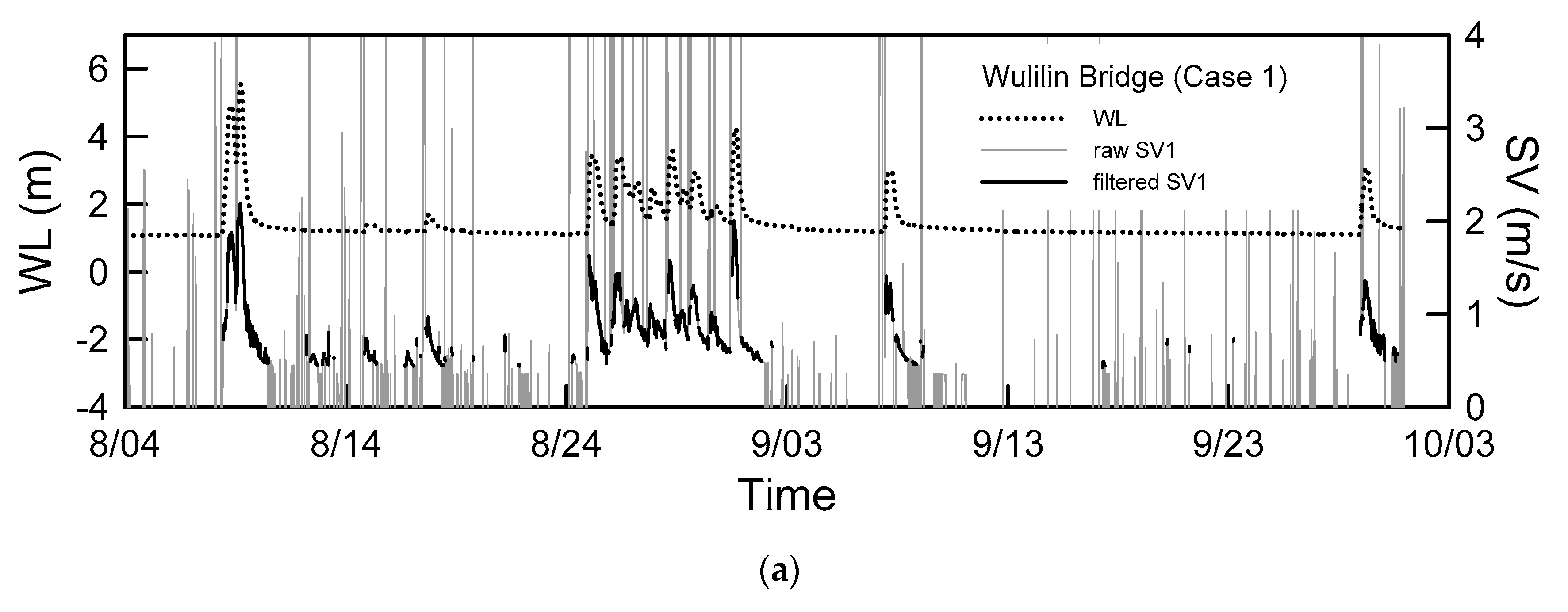
The Doppler effect has been applied to SVR to measure the ripple speed on the water surface. The ripple speed is assumed to be the same as water SV. Radar wave frequency is altered as signals are reflected from moving ripples, and the difference in frequency is observed between transmitted and reflected signals. Therefore, when the water slope is too mild and at low WL or under strong wind conditions, the frequency shift is affected, as illustrated by the conspicuous noise and spikes shown in Figure 1. The SV data shown in Figure 1 were collected from the Wulilin Bridge hydrological station during rainfall season in 2015. SV data with excess noise are unsuitable for subsequent analysis or assimilation into a hydraulic numerical model for a flooding warning system.
Several despiking methods for the postprocessing of data obtained using the variety of hydraulic instruments, such as acoustic Doppler velocimeters (ADVs) used for measuring mean and turbulent components, have been studied. Spikes in records may be from multiple sources. Goring and Nikora [16] combined three concepts for despiking ADV data: differentiation enhances the high-frequency portion of a signal, the universal threshold yields the expected maximum of a random series, and a good data cluster in a dense cloud in phase space. Mori et al. [17] compared the method developed by Goring and Nikora [16] with the classical low correlation method when eliminating the spike noise of ADV recorded data in bubbly flow. Islam and Zhu [18] developed an iteration-free despiking algorithm for highly contaminated ADV data by applying a bivariate kernel density function and its gradient to separate the data cluster from the spike clusters.
To eliminate the influence of wind-drift current, Fukami et al. [14] used a linear equation function of wind velocity above the water surface to modify SV data. Fulton [19] provided guidelines for setting-up and operating the SVR. The study highlighted that when collecting SV data, the user should avoid wind-dominated reaches, eddies, secondary flows, and macro turbulence. Filtering schemes such as high- and low-pass filters, moving averages, local polynomial regression fitting (LOESS), Savitsky–Golay filters, and Kalman filters have been suggested to reduce the noise. However, the diagnostic tests required for current meters and acoustic instruments are unavailable for SVRs. Some SVRs produce spectra, which offer a quantitative tool that serves as a “spin test” for electromagnetic instruments and can be used to qualify the value of estimated SV. The nature of each spike in raw SV data is too complex to easily identify filtering criteria. In addition, even when two SVRs are only a few meters apart above the thalweg, the variation of the two signals may be significantly different. SVR signals may be influenced by the surrounding environment, such as an opened water gate or flow pipe. Identifying the true SVR signal in situ can be problematic under such environments. Thus, filtering spikes or noise in the data by setting a threshold is unsuitable. If SVR is the instrument used for computing continuous flow discharge, a method must be developed and assessed for filtering the noise in its signals.
Several methods have been developed for smoothing continuous data and filtering spikes or noise, such as moving average (MA), robust LOESS (RLOESS) proposed by Cleveland [20], locally weighted scatterplot smoothing (LOWESS) proposed by Cleveland and Devlin [21], and the Savitzky–Golay (SGLOLAY) filter proposed by Savitzky and Golay [22]. The last three methods are based on least squares regression and feature the flexibility of nonlinear regression. Through localized data subsets, a function is constructed to describe data variation in each point. Input requirements include polynomial models, bandwidth, smoothing parameters, and weight function. RLOESS can be used to reduce outliers in some iterations, with an emphasis on overcoming extreme outliers if too many are present. In this study, the performance of these smoothing methods was evaluated.
In this study, SV data from the Wulilin Bridge and Yenfong Bridge hydrological stations at the Dianbau River in Southern Taiwan were analyzed. The Dianbau watershed is an experimental watershed constructed by the Water Resources Planning Institute in cooperation with the Taiwan Typhoon and Flood Research Institute (TTFRI) for establishing monitoring stations. In the watershed, hydrological monitoring includes WL radar, continuous SVR for water SV, and urban flooding monitoring through a pressure-type gauge. Noncontact measurement methods for calculating discharge in rivers have been studied. A WL radar gauge and two continuous SVRs for surface wave velocity were established to estimate discharge through the velocity index method. ADCP data during a typhoon were obtained for determining the index velocity with water stages. The discharge data obtained from these sites were used for calibrating local runoff models and for upstream boundary condition of river routing models.
The Wulilin Bridge station is located downstream of the Dianbau River and has a channel slope of approximately 1/805. After channel regulation, the cross-sectional shape of the Dianbau River at Wulilin Bridge is trapezoidal, with a topline width of approximately 40 m. The Yenfong Bridge station is located upstream of the Dianbau River, with an average cross-sectional width of 27 m; at the Yenfong Bridge station, the channel slope is approximately 4/135, which is 23.8 times that at Wulilin Bridge station. The WL gauge and two SVRs were constructed on the upstream side of the bridge. Neither bridge has piers.
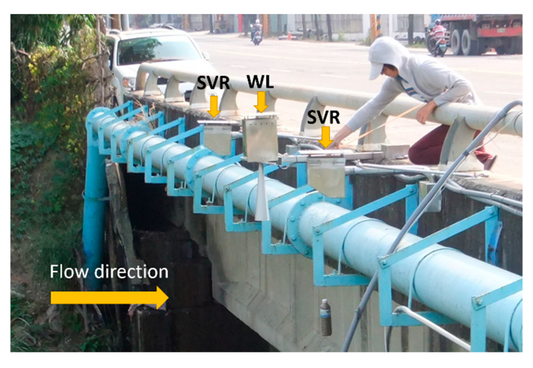
Two fixed SVRs, which were both Sommer RG30s [23], were installed besides one WL radar on the bridge desk, as shown in Figure 2. The radar devices had a signal frequency of 24 GHz (K-band) and a measuring range of 0.15–15 ms−1. The installed WL radar at Wulilin Bridge had a 10-min sampling rate and was constructed by the Water Resources Agency. The two SVRs at the Wulilin Bridge and the one WL radar and two SVRs at Yenfong Bridge with 1-min sampling rates were constructed by TTFRI. Five-year SV and WL data at the sites were collected. The data of the first 3 years were used for creating data relationships, and data from the last two years were used for evaluating the performance of the proposed method.
2. Methods
2.1. Statistic Method
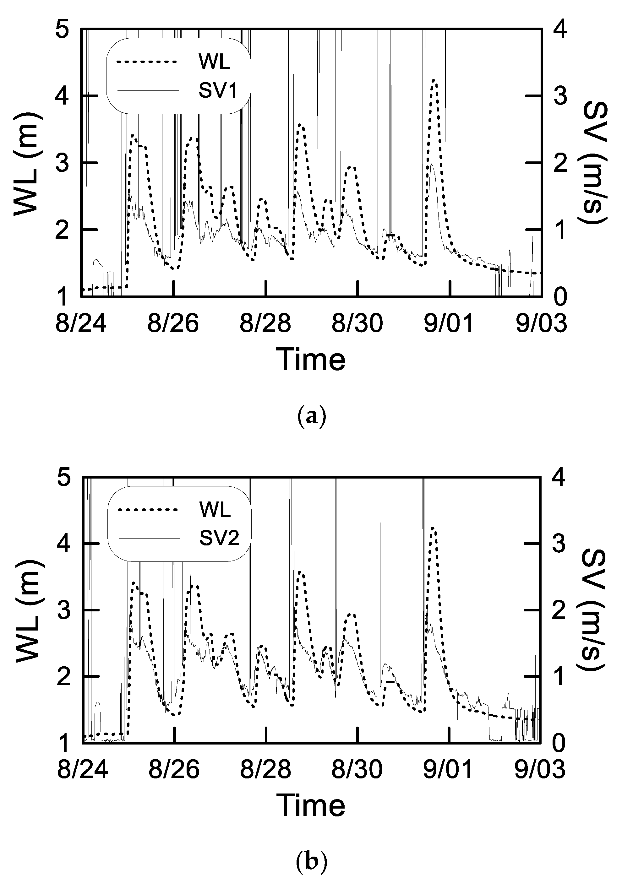
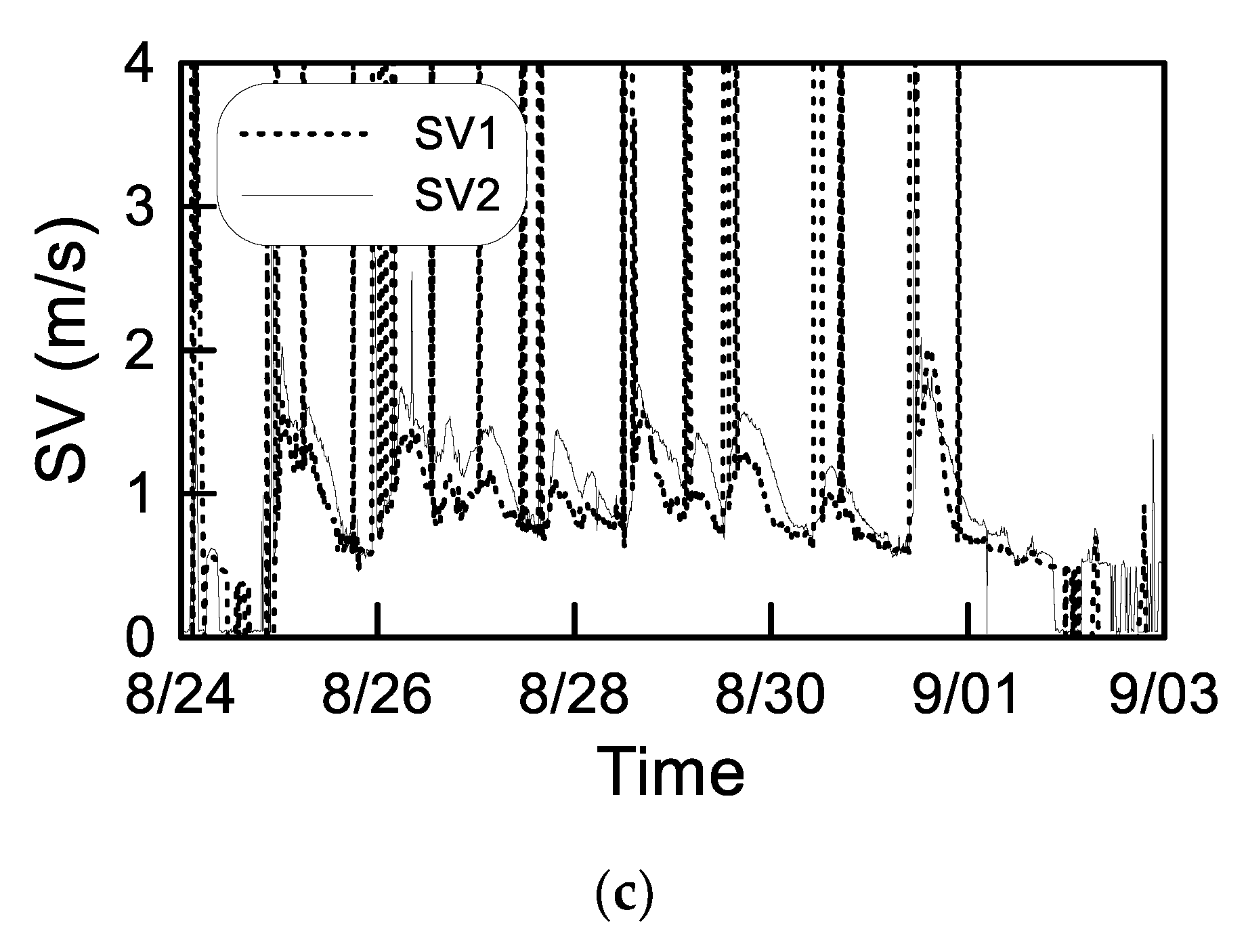
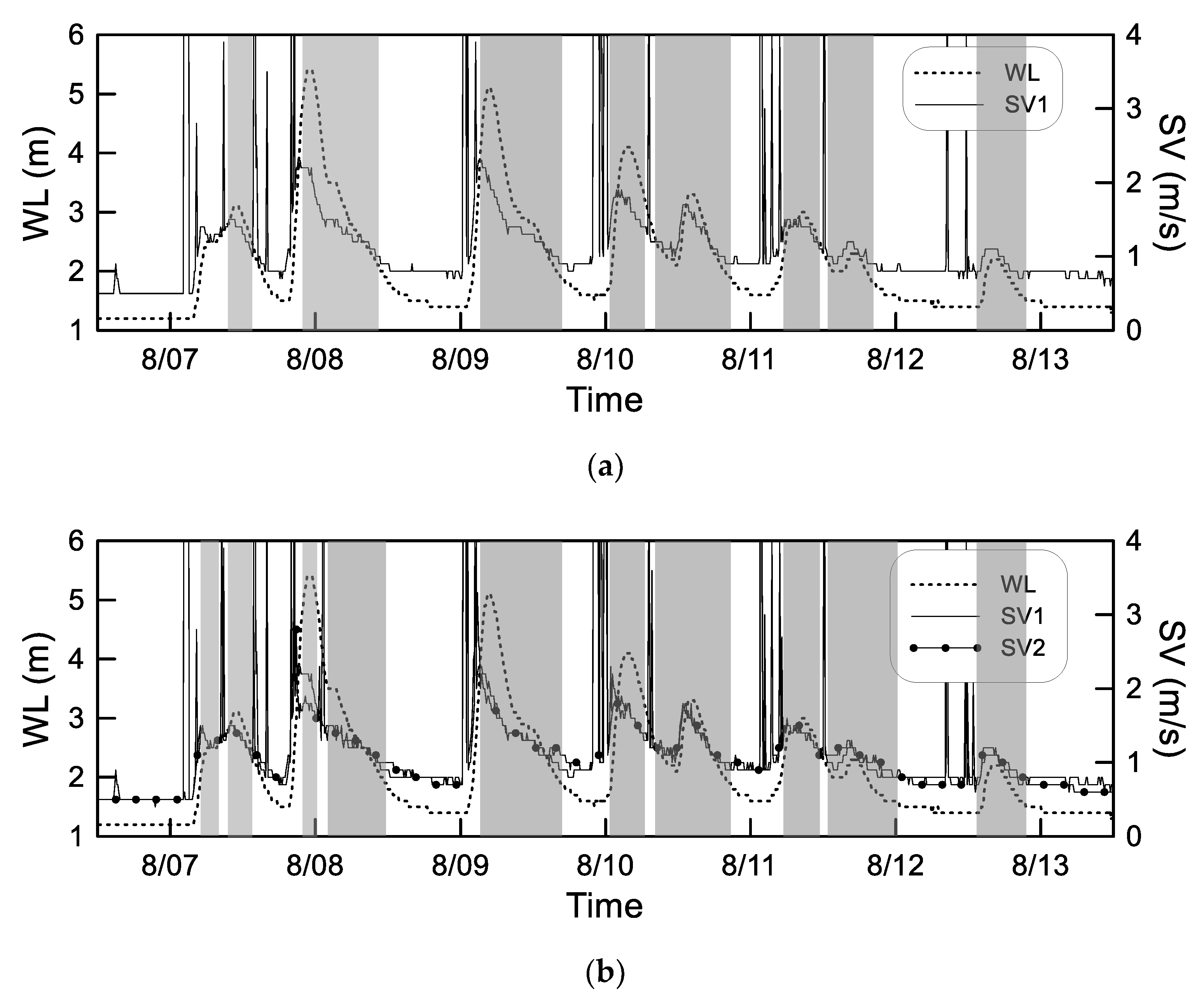
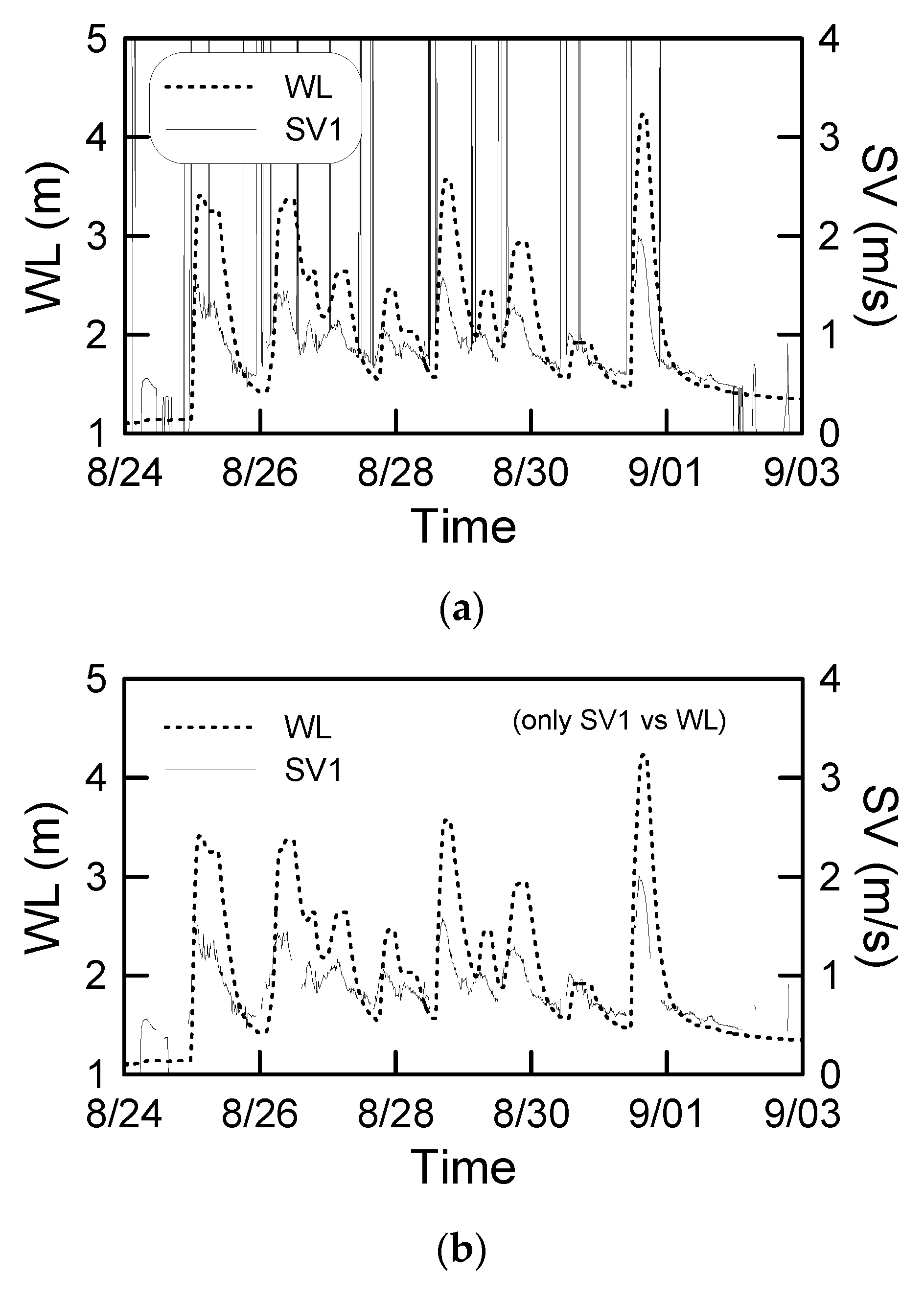
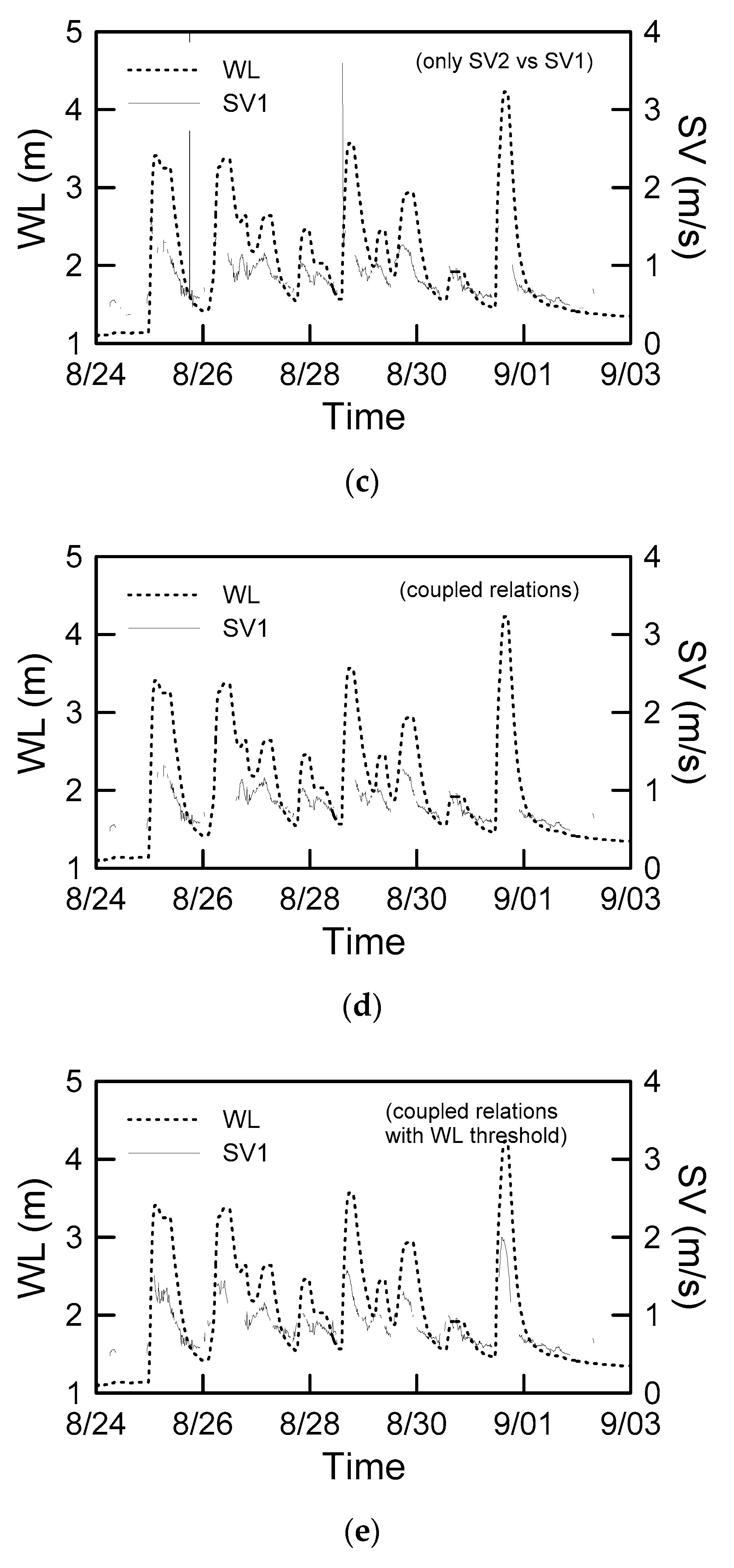
Although SV and WL are different flow features, some dependences exist between the two, as illustrated by the time series of WL and SV in Figure 3. The two SV values exhibit a similar trend with WL values, as shown in Figure 3a,b. Figure 3c reveals that the two SV values exhibit a similar trend.
The value of SV data at a certain WL has been shown to always differ due to the WL rising process, falling process, or uncertainty of each event, but it varies within a limited area, which is similar to flow acceleration and deceleration during the passage of a flood wave [1,24]. In the present study, a prediction interval (PI) method [25] was applied to filter continuous SV data. PI is often used in regression analysis. Observed data are used for estimating an interval where future observations will fall with a certain probability. This is based on the sample mean and the sample variance ; thus, the (1 − α)100% two-sided PI is expressed as
where n = sample quantity and = the t-value corresponding to n − 2 degrees of freedom. The (1 − α)100% prediction interval, most commonly a 95% PI in hydraulics, was used in this study. The value on the regression line is determined by inputting future observation data xh. Sxx = the sum of squares of the difference between each x and .
Basic regression models such as linear, power law, log law, and exponential regressions are used as follows:
where (x, y) is the independent data vector, and a, b, and c are parameters in each model. In this study, the least absolute residual [26] approach was used for obtaining parameters.
Two types of physics relations—SV versus WL and the relation between the two SVRs—were established at the two stations. Therefore, three relations were constructed: SV1 versus WL, SV2 versus WL, and SV2 versus SV1. The three independent data sets were acquired separately.
2.2. Data Sampling
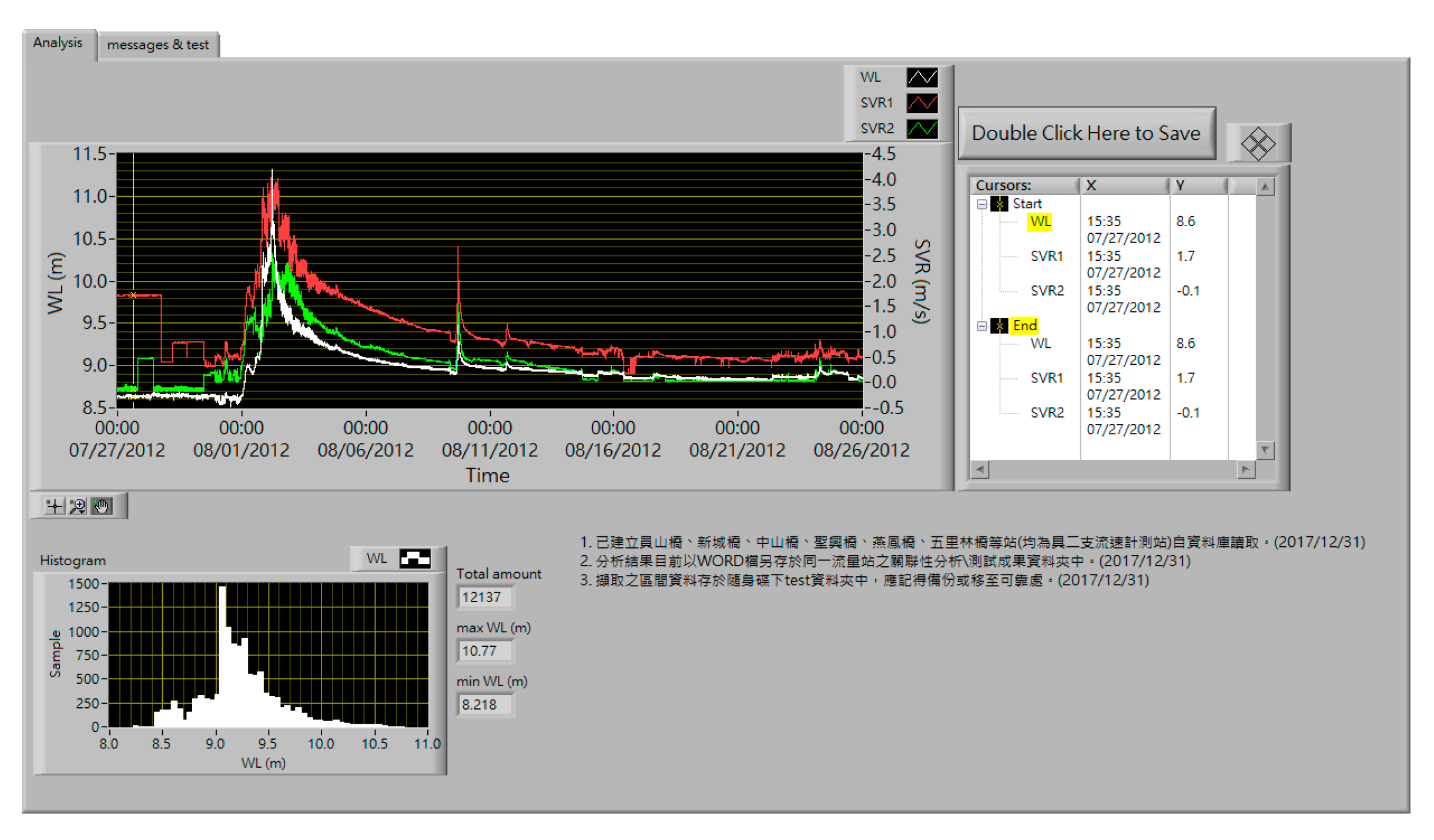
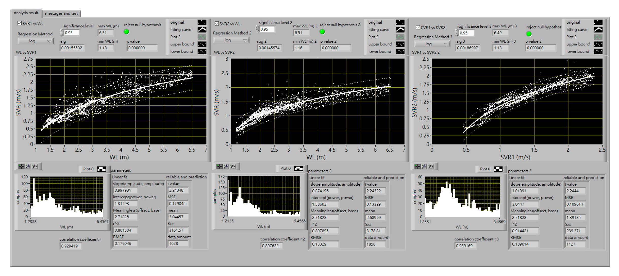
Data quality, data distribution, and sufficient samples size are vital for statistical analysis. Moreover, the noise in sampled data should be detected because this may influence the results. If data distribution is extremely non–uniform, or it does not cover the low and high WLs that represent the samples, the data distribution is insufficient. Sampling from big data is therefore necessary before establishing regression relations, and the samples should be carefully selected from conspicuous noises. The human–machine interface program shown in Figure 4 was developed using the graphical language of LabVIEW for selecting data periods. The software program integrates the data from Water Resources Agency and TTFRI and depicts the overall time series of data. A user can zoom in, zoom out, and drag the time series of data to a relevant area. The data histogram is refreshed instantly and compared with different WLs because the data period is selected to display data distribution; however, identifying physical homogeneity is still difficult [27]. After selecting the samples set, the regression results of each samples set and its relevant prediction parameters are calculated, as shown in Figure 5.
Figure 6 presents SV and WL data of heavy rain days at the Wulilin Bridge in 2012. Both trends appear profoundly dependent, apart from spikes and SV data at low WL. The gray color depicts a less noisy region, from which the samples may be selected for further analysis. The criteria for selecting SV data and establishing SV versus WL regression are as follows:
- The variations of SV and WL are similar during the same period.
- Conspicuous spikes should be excluded.
- The SV data at low and flat WLs that look unnatural should be excluded, such as those observed in the afternoon of August 8 and at midnight of August 12 in the blanking area in Figure 6a.
- If the SV data at a specific WL were sampled more than other WLs from the histogram, the SV data at the same WL would not be acquired thereafter.
- If the SV data amount at low and medium WLs is sufficient as indicated by the histogram, the lower WL events could be ignored and focus on only the higher WL events.
The criteria for selecting SV data and establishing SV2 versus SV1 regression are as follows:
- The variations of SV1 and SV2 are similar in the same period, both trends exhibiting little difference with WL, such as those observed in the morning and night of August 7 and the afternoon of August 10, as shown in Figure 6b.
- If either SV1 or SV2 spikes exist, the data are excluded from the samples.
- If the SV data at a specific WL are sampled more than other WLs, the SV data at the WL would not be acquired thereafter.
- If the SV data amount at low and medium WLs is sufficient as indicated by the histogram, the lower WL events could be ignored and focus on only the higher WL events.
3. Results and Discussion
3.1. Samples Quality
The samples information of the three relations, SV1 versus WL, SV2 versus WL, and SV2 versus SV1, at the Wulilin Bridge and Yenfong Bridge selected from 2012–2014 are listed in Table 1 and Table 2, respectively. The total amount of data collected at the Wulilin Bridge and Yenfong Bridge for establishing the three relations ranged from 1127 to 1858 and 10,987 to 15,649, respectively. One order-total difference existed between the two data sets obtained from the stations due to the WL sampling rate, as mentioned in the introduction section. All the correlation coefficients (r) were over 0.7, indicating a high correlation in each data set. The p value [28] of each case was calculated to ascertain if the null hypothesis was rejected. The p value based on Pearson type distribution with 0.05 significance level for all cases was calculated to evaluate whether the null hypothesis is rejected. The p value of all cases in this study was zero. A small p value suggests that the alternative hypothesis is true; thus, the test is highly significant.
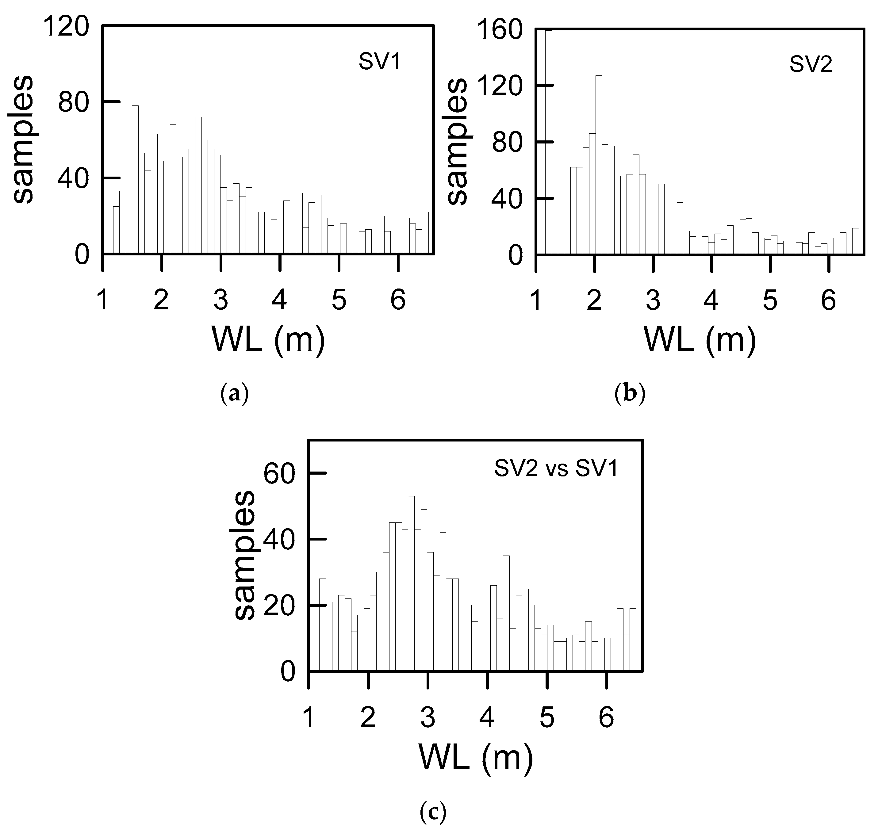
An example of the acquired SV data distribution with the WL of each data set at the Wulilin Bridge is presented in Figure 7. Data were evaluated for outliers to maintain a homogenous distribution, thus improving the regression model. Despite selecting high-WL data from several flooding events, the samples for high WL remained low because high-WL periods during flooding events are short.
3.2. Evaluation of the Different Regression Models
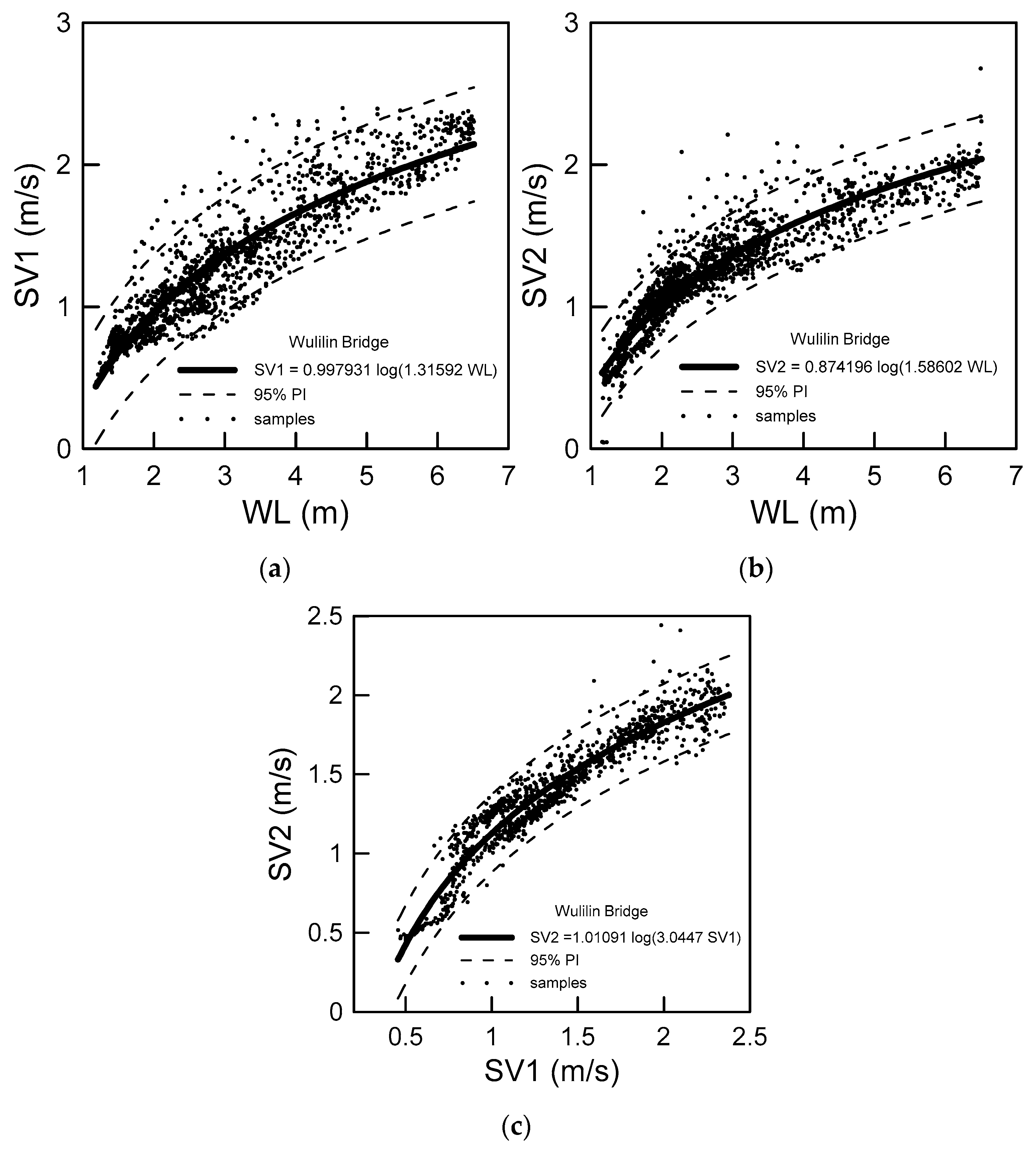
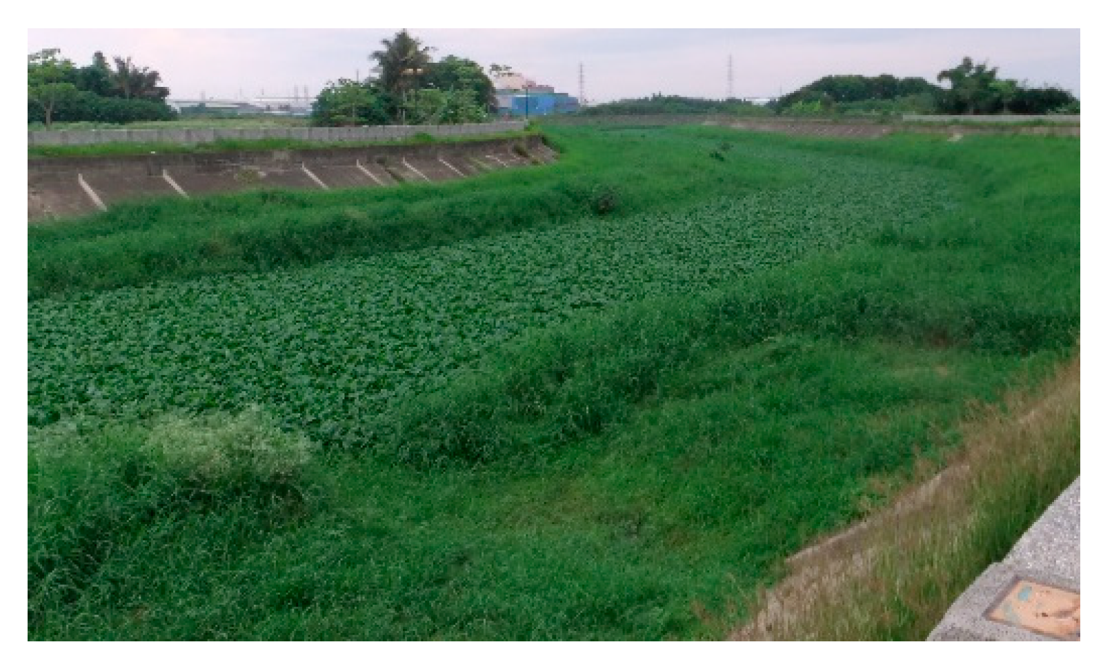
Four simple regression models, namely linear, power law, log law, and exponent, were applied to each sample set at the Wulilin Bridge and Yenfong Bridge. The deterministic factors, R2, of these bridges are shown in Table 3 and Table 4, respectively, and they indicate the goodness of fit for each regression result. In the Wulilin Bridge cases, all the goodness of fit results for SV1 versus WL were similar. The goodness of fit of the log law regression result of SV2 versus WL and SV1 versus SV2 exhibited the best fit. Finally, the log law regression results and its relative PI information for each sample were selected for filtering performance testing. The scatter plot and log law regression result with its 95% PI of each samples set at the Wulilin Bridge are depicted in Figure 8. In the SV1 versus WL and SV2 versus WL cases, few points below 5 m WL deviated from the upper bound of PI. Data above the regression line were sparser than that below the line because the flow acceleration during the rising process was unstable and vegetation was present on the riverbed. In Figure 9, the water hyacinths are shown to cover the entire channel bed. Fewer data in SV2 versus SV1 data set were separated from the PI, indicating similar phenomenon measurements in situ.
Three relations were first explored: only SV1 versus WL relation, only SV2 versus SV1 relation, and coupled SV1 versus WL and SV2 versus SV1. The filtered SV results and comparisons were nearly identical in SV1 and SV2; thus, only the SV1 data of each site will be discussed hereafter. Heavy rains on August 24–September 2 in 2015 at the Wulilin Bridge station (Figure 10) were used to explain each relation’s performance. Considerable noise and spikes existed in the raw SV data, as shown in Figure 10a. Satisfactory results were obtained using only the SV1 versus WL relation, although noise was evident at low WL (Figure 10b). By contrast, the noise at low WL was filtered by using only the SV2 versus SV1 relation. Many standard data seemed filtered, but a few spikes present in the data may have been caused by the spikes occurring in SV1 and SV2 at the same time (Figure 10c). Combining the two relations to treat the data filtered all the noise at the expense of the standard data (Figure 10d). By merging the advantage of two relations by roughly establishing a WL threshold, the relation between the two SVs was used as the WL below the WL threshold, as shown in Figure 10e. The threshold in this preliminary study is estimated by looking for a WL that is higher with the least noise. The SV data quality is influenced by the environment, including the water slope, the bed roughness, and wind conditions etc. The threshold implies selecting a WL where SV data is less influenced by bed roughness and close to the riverbed elevation. Subsequently, more data at higher WLs were reserved, and the noises at low WLs were filtered. Figure 11 presents the final results from the coupled relations, with approximate WL thresholds of 1.5 m and 20.0 m at Wulilin Bridge and Yenfong Bridge, respectively, demonstrating that satisfactory results were obtained.
The detection rate = nn/nTs, nn = the amount of noise data after filtering, nTs = the total amount of samples, was used to realize the total amount of filtered data in different relationships. Although slight over-sifting standard data and miss-sifting abnormal data were unavoidable by using this method, evaluation of model performance by using the detection rate still offered a method to understand performance roughly. The last results of each case at the Wulilin Bridge and Yenfong Bridge are listed in Table 5 and Table 6, respectively. The first case was the entire rainfall season in 2015, which was used to evaluate the overall performance, including low WL and rainfall periods. The last four cases were rainfall events in which the WL was raised by at least 4 m or when it rained over many days. Cases 2 and 3 were covered in Case 1 to realize the filtering difference between overall days and rainfall days. The highest WL of Cases 4 and 5 was higher than that of the samples. Overall, the detection rate of the relation between the two SVs was much higher than that of SV versus WL. The detection rate of the coupled relations was slightly higher than that of the uncoupled SVs relation, suggesting that the detected questionable data of the relation between the two SVs almost covered the detected data of SV versus WL. For the three relations, the detection rate in Case 1 was much higher than that in Cases 2 and 3, which meant most of the data were detected during low WL. If only the SV data at low WL were processed by the relation between the two SVs, the standard data at higher WL would not be over-filtered. The detection rate was lower with the WL threshold than without the WL threshold, but it was slightly higher than that of the SV versus WL relationship.
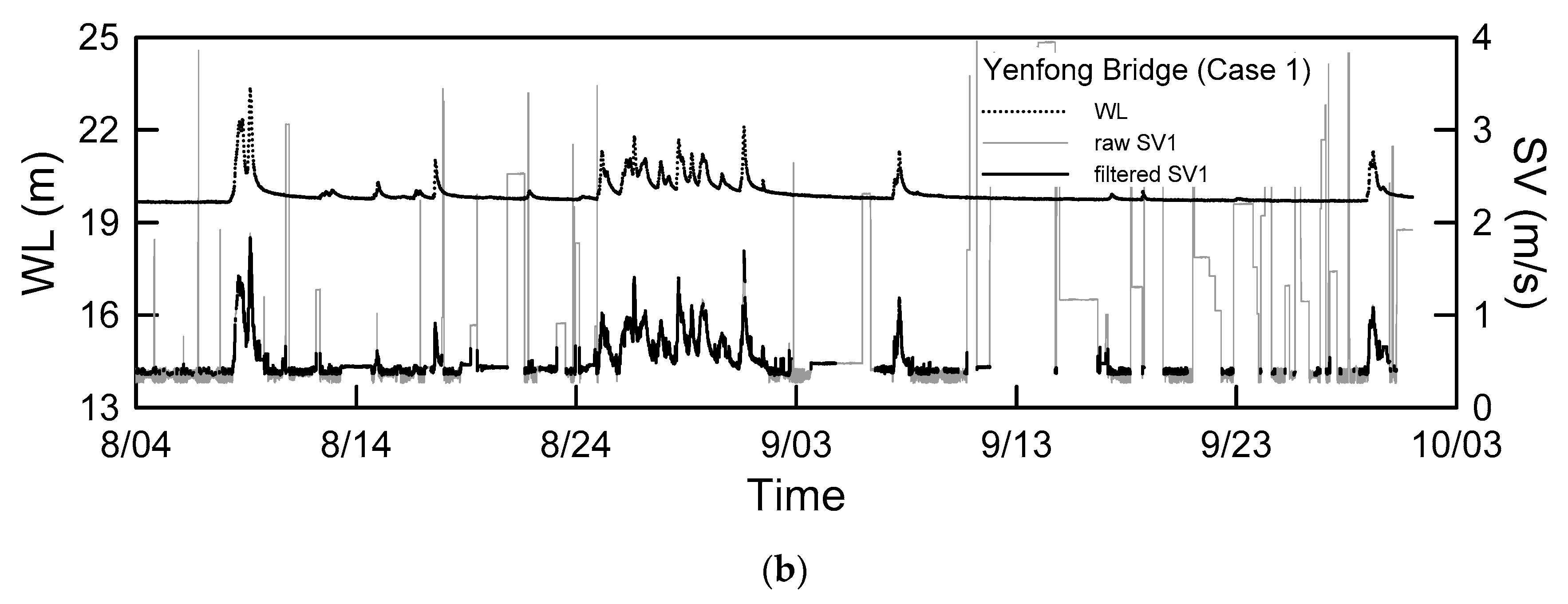
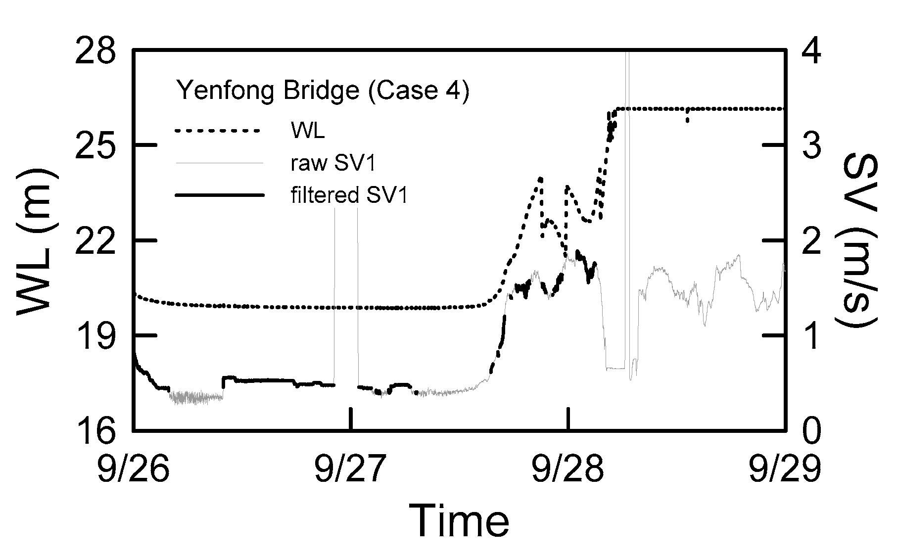
The detection rate of each case at the Yenfong Bridge station was much lower than that at the Wulilin Bridge station, whereas the PI relationships were similar. Lower detection was attributed to the steeper channel slope, which led to apparent ripples on the water surface. Moreover, the detection rate of SV2 in Cases 4 and 5 abnormally reached 100%, as illustrated in the time series of SV in Figure 12. The WL at Yenfong Bridge was above the bridge bottom level of 25.5 m and hit the WL radar and two SVRs. As a result, this equipment could not function well at the time, yielding questionable data. Although the equipment was repaired after the specified event, SVR2 did not function accurately, as indicated by the 100% detection rate in Case 5.
3.3. Comparison of Proposed Filter Method and Modern Smoothing Methods
The difference between the result obtained using the method developed in this study and using some modern smoothing methods, particularly RLOESS and robust LOWESS (RLOWESS) methods, was evaluated, and the results emphasized their despiking ability. A Matlab function was implemented in each smoothed result for the data from five cases at Wulilin Bridge. The default polynomial degree and iteration time settings of LOESS, RLOESS, LOWESS, RLOWESS, and SGLOLAY filter functions were used. The polynomial degree was the second and first orders of LOESS and LOWESS, respectively, and the iteration time of RLOESS and RLOWESS was five. Three bandwidths of 0.1%, 0.5%, and 1% of the total data amount were tried for the smoothing effect. One percent data amount was approximately 71 data points in the Wulilin Bridge cases. The difference with sorted data determined using normalized root-mean-square-error (RMSE) is presented in Table 7. The extreme WL variation range in each case was different; the RMSE result was normalized by dividing the maximum water depth. The smallest normalized RMSE in each case and each method occurred randomly, which made it difficult to distinguish.
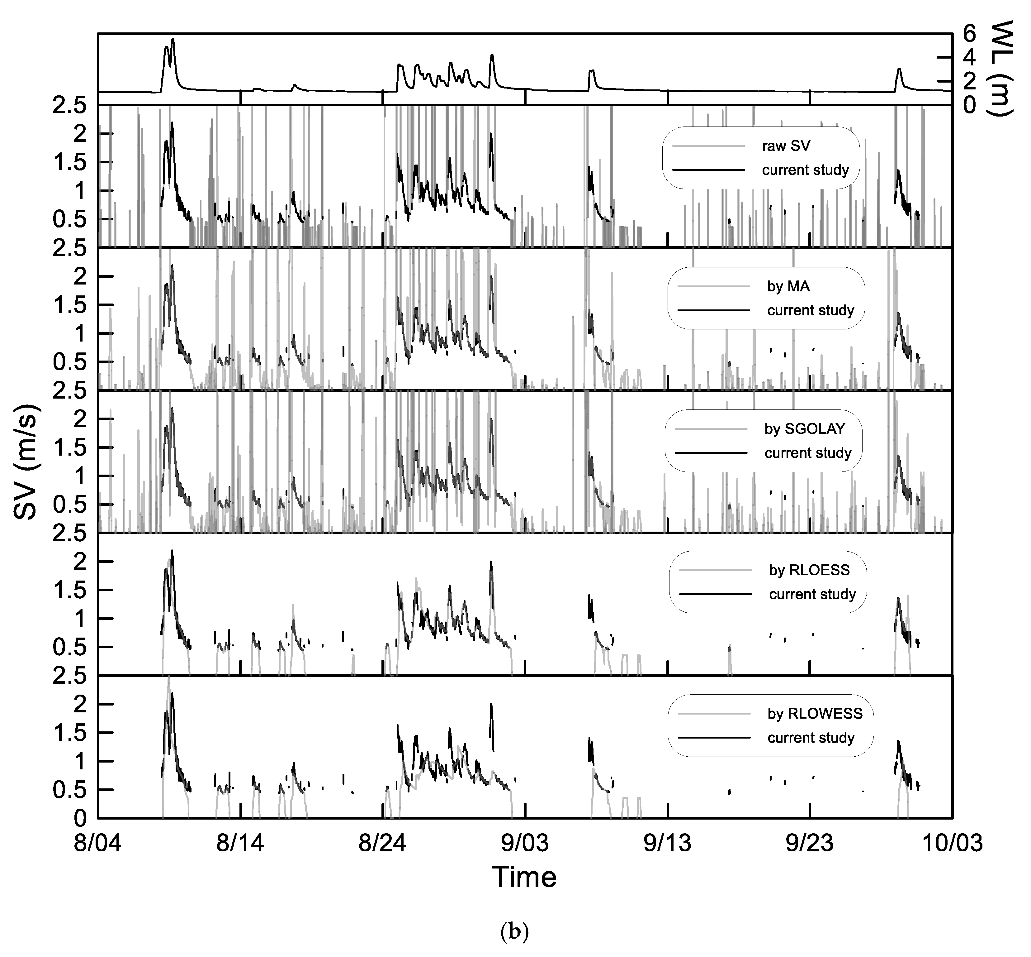
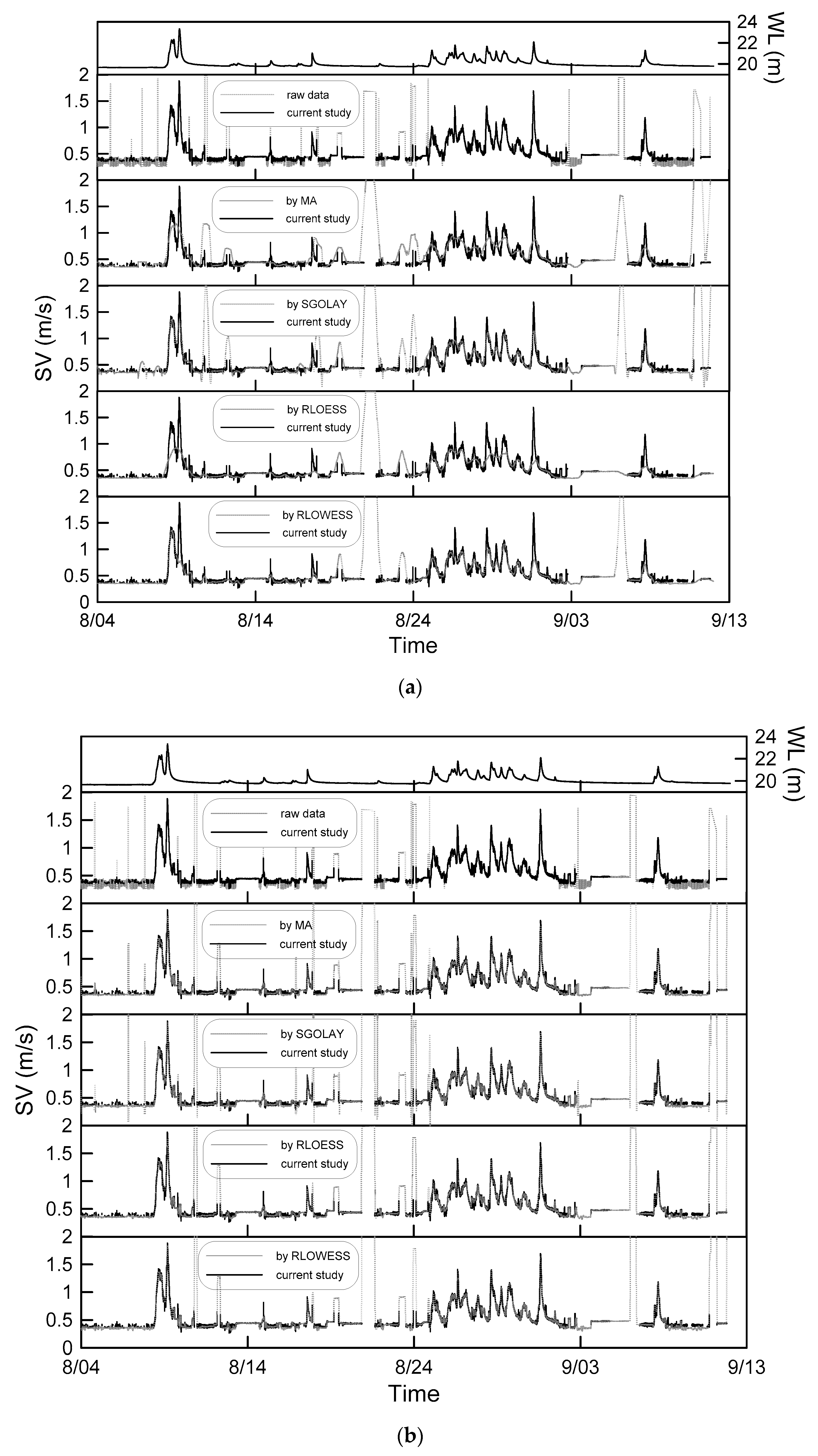
From the analysis, the narrower the bandwidth, the closer the smoothed result is to the original time series of the data, and the wider the bandwidth, is the finer the smoothing, such that the noise and spikes contaminated the overall effect. Figure 13 depicts the time series of SVs from the largest and smallest bandwidths of 1% and 0.1% at the Wulilin Bridge. The result obtained through the filtering of raw data by using the method proposed in this study is represented by the first graph in the figure, with the filtered data plotted below the initial graph. The wider bandwidth influenced the performance of MA and SGOLAY, and more noise was generated by the original spikes, as shown in Figure 13a. The performance of the LOESS and LOWESS methods was similar to that of SGOLAY. Although the SV spikes at low WL were depressed, the SV data at high WL processed using the MA, SGOLAY, RLOESS, and RLOWESS methods were severely contaminated. Produced noise lower than the general value by SGOLAY method may have been induced by higher order polynomial. RLOESS and RLOWESS produced satisfactory results. For RLOESS and RLOWESS, noise and spikes at low WL disappeared, and the overly far flat SV data occurred during flooding periods, such as the period from August 24–September 3. The smallest bandwidth case yielded similar results and performance during August 24–September; thus, the results of RLOESS and RLOWESS seemed superior, as shown in Figure 13b. The result of RLOESS and RLOWESS could be applied to estimate discharge using the index velocity method because most noise and spikes were filtered.
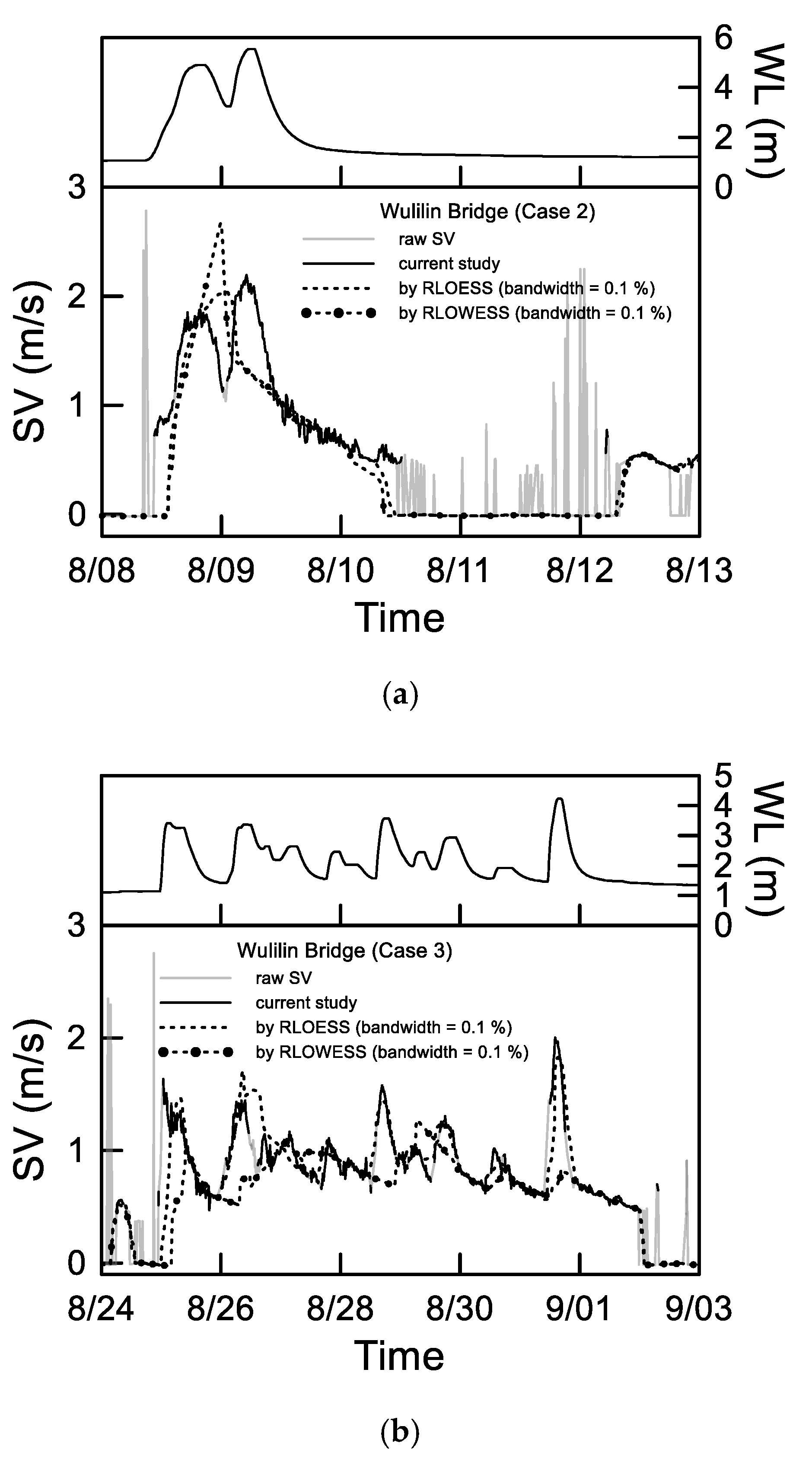
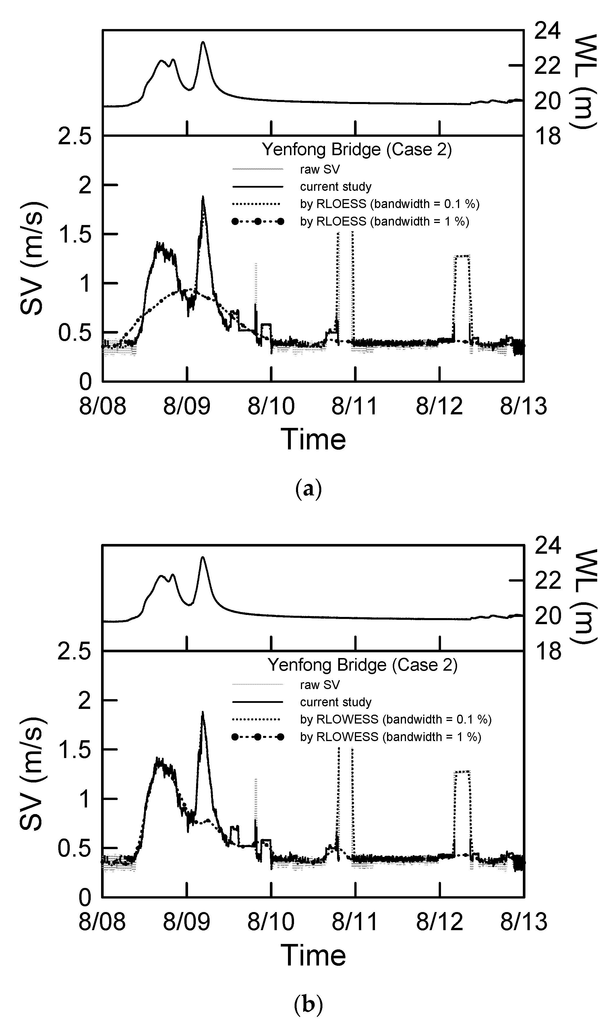
This study focused on the smoothed result under high-WL conditions. The local variations, Cases 2 and 3, analyzed using RLOESS and RLOWESS with a narrow bandwidth of 0.1% are plotted in Figure 14a,b, respectively. As shown in Figure 14a, two peaks were observed in WL and SV during the two rainy days in Case 2. Neither method could describe the SV variation around the peak. RLOESS smoothed the variation into one peak, whereas RLOWESS over-smoothed the data much higher than the original at midnight on August 9. The SV data at low WL was almost despiked to zero by both methods. Moreover, the SV at low WL always had a low speed in situ, with the zero value out of the range described by the manufacturer; thus, the SV value could be validated by the proposed method and smoothing methods. Several random peaks were present over a week during rainy days (Figure 14b). RLOESS outperformed RLOWESS and captured several peaks. The line acquired by RLOWESS appeared smooth over these peaks, even at the single peak on September 1, which suggested that these spikes were sorted as spikes and were filtered. As shown in Figure 14b, on August 24, both methods were inaccurate, producing a single peak when the WL was not rising. As shown in Figure 14b, near midnight on August 24, the result of both methods was contaminated by spikes.
The riverbed slope at the Yenfong Bridge is much steeper than that at the Wulilin Bridge, and the data sampling rate was tenfold. The number of spikes in the raw data at the Yenfong Bridge during the same period was much lower, and it infers the ripples on the water surface, always accompanied with the flow, and not easily influenced by the environment. The effects of 0.1% and 0.01% bandwidths were similar; thus, we presented only 0.1% and 1% bandwidth cases. The results with the two bandwidths of 1% and 0.1% for the overall rainfall season in 2015 are shown in Figure 15. The 1% data amount was approximately 770 points; therefore, approximately 77 points in the 0.1% bandwidth case were also tested for comparison with the result of Wulilin Bridge case. In the 1% bandwidth case, spikes were smoothed at low WL of each case, and the results of RLOESS and RLOWESS were satisfactory. However, too many continuous spikes existed and remained. The trace of smoothed data at flooding peaks could still be observed in each case and was further evident in Case 2, as shown in Figure 16. Reducing the bandwidth by ten times (0.1%) retained the spikes for ordinary days, and the methods lost their filtering ability. RLOWESS offered superior performance, despite filtering the second peak on August 9.
The performance of the smoothing methods was found to be mainly influenced by the noise ratio in the raw data, length of spikes, bandwidth of the smoothing method, and occurrence frequency of multi–peaks during a flooding event. RLOESS and RLOWESS performed well, although concluding which method is superior is challenging because both methods were limited in treating data with too much noise.
4. Conclusions
In this study, a human–machine software written by the authors was used for sorting continuous raw SV and WL data. Findings of such analysis are crucial in establishing regression relationships and their PI for filtering noises and spikes. Two data sets from different sites were applied to evaluate the performance of the model by using different regression relationships and coupled relationships. The coupled relations, SV versus WL relation and the relation between the two SVs with an approximate WL threshold, exhibited the most accurate result and were selected for advanced analysis. Several cases of data were used to test the detection rate and smoothing by modern smoothing methods. In a reasonable data set in which fewer spikes existed in the SV data, RLOESS and RLOWESS offered superior performance, particularly with the appropriate bandwidth. Determining the superior method is still challenging because all the smoothed data were contaminated by noise due to the presence of too much noise or subtle flooding peaks. The noise–signal ratio, length of spiking, decision of bandwidth, and data sampling rate were all revealed to be major factors. The present study offered an excellent sorting of continuous SV data. Although errors were still observed, most noises and spikes were filtered, and the distortion of raw data was avoided for their use in advanced analysis. The WL threshold criteria and, the proposed method will be applied at different sites in future studies.
Author Contributions
H.W. conceived and designed the methodology, data curation, writing software, analyzed the data. G.F. gave some significant suggestions. S.T. spent effort on reviewing and editing this article. J.H. performed the data smoothing for comparing with the results by the proposed method, gave suggestions. All the authors contributed to the writing and editing of the manuscript.
Funding
This work was partly supported by Water Resources Planning Institute, Water Resources Agency, Ministry of Economic Affairs (Project No. MOEAWRA1060123), and was partly supported by TAIWAN SECOM CO., LTD.
Acknowledgments
The authors thank the anonymous reviewers for the constructive comments. This manuscript was edited by Wallace Academic Editing.
Conflicts of Interest
The authors declare no conflict of interest.
References
- Aberle, J.; Rennie, C.D.; Admiraal, D.M.; Muste, M. Experimental Hydraulics: METHODS, Instrumentation, Data Processing and Management—Volume II: Instrumentation and Measurement Techniques; CRC Press: Boca Raton, FL, USA, 2017. [Google Scholar]
- Rantz, S.E. Measurement and Computation of Streamflow—Volume 2, Computation of Discharge; US Department of the Interior, Geological Survey: Reston, VA, USA, 1982; p. 373. [Google Scholar]
- Hidayat, H.; Vermeulen, B.; Sassi, M.G.; Torfs, P.J.J.F.; Hoitink, A.J.F. Discharge estimation in a backwater affected meandering river. Hydrol. Earth Sys. Sci. 2011, 15, 2717–2728. [Google Scholar] [CrossRef]
- Hoitink, A.J.F.; Buschman, F.A.; Vermeulen, B. Continuous measurements of discharge from a horizontal acoustic Doppler current profiler in a tidal river. Water Resour. Res. 2009, 45, W11406. [Google Scholar] [CrossRef]
- Nihei, Y.; Kimizu, A. A new monitoring system for river discharge with horizontal acoustic Doppler current profiler measurements and river flow simulation. Water Resour. Res. 2008, 44, W00D20. [Google Scholar] [CrossRef]
- Sassi, M.G.; Hoitink, A.J.F.; Vermeulen, B. Discharge estimation from H-ADCP measurements in a tidal river subject to sidewall effects and a mobile bed. Water Resour. Res. 2011, 47, W06504. [Google Scholar] [CrossRef]
- Fujita, I.; Muste, M.; Kruger, A. Large-scale particle image velocimetry for flow analysis in hydraulic engineering applications. J. Hydraul. Res. 1998, 36, 397–414. [Google Scholar] [CrossRef]
- Fujita, I.; Tsubaki, R.; Deguchi, T. PIV measurement of large-scale river surface flow during flood by using a high resolution video camera from a helicopter. In Proceedings of the 3rd Hydraulic Measurements and Experimental Methods Conference, Lake Placid, NY, USA, 10–12 September 2007; pp. 344–349. [Google Scholar]
- Costa, J.E.; Spicer, K.R.; Cheng, R.T.; Haeni, F.P.; Melcher, N.B.; Thurman, E.M.; Plant, W.J.; Keller, W.C. Measuring stream discharge by non-contact methods: A proof-of-concept experiment. Geophys. Res. Lett. 2000, 27, 553–556. [Google Scholar] [CrossRef]
- Costa, J.E.; Cheng, R.T.; Haeni, F.P.; Melcher, N.; Spicer, K.R.; Hayes, E.; Plant, W.; Hayes, K.; Teague, C.; Barrick, D. Use of radars to monitor stream discharge by noncontact methods. Water Resour. Res. 2006, 42, W07422. [Google Scholar] [CrossRef]
- Plant, W.J.; Keller, W.C.; Hayes, K.; Spicer, K. Streamflow properties from time series of surface velocity and stage. J. Hydraul. Eng. 2005, 131, 657–664. [Google Scholar] [CrossRef]
- Fulton, J.W.; Ostrowski, J. Measuring real-time streamflow using emerging technologies: Radar, hydroacoustics, and the probability concept. J. Hydrol. 2008, 357, 1–10. [Google Scholar] [CrossRef]
- Chiu, C.L. Velocity distribution in open channel flow. J. Hydraul. Eng. 1989, 115, 576–594. [Google Scholar] [CrossRef]
- Fukami, K.; Yamaguchi, T.; Imamura, H.; Tashiro, Y. Current status of river discharge observation using non-contact current meter for operational use in Japan. In Proceedings of the World Environmental and Water Resources Congress 2008: Ahupua’a, Honolulu, HI, USA, 12–16 May 2008. [Google Scholar]
- Corato, G.; Moramarco, T.; Tucciarelli, T. Discharge estimation combining flow routing and occasional measurements of velocity. Hydrol. Earth Syst. 2011, 15, 2979–2994. [Google Scholar] [CrossRef]
- Goring, D.G.; Nikora, V.I. Despiking acoustic Doppler velocimeter data. J. Hydraul. Eng. 2002, 128, 117–126. [Google Scholar] [CrossRef]
- Mori, N.; Suzuki, T.; Kakuno, S. Noise of acoustic Doppler velocimeter data in bubbly flows. J. Eng. Mech. 2007, 133, 122–125. [Google Scholar] [CrossRef]
- Islam, M.R.; Zhu, D.Z. Kernel density-based algorithm for despiking ADV data. J. Hydraul. Eng. 2013, 139, 785–793. [Google Scholar] [CrossRef]
- Fulton, J.W. Guidelines for Siting and Operating Surface-Water Velocity Radars. Available online: https://my.usgs.gov/confluence/display/SurfBoard/Guidelines+for+Siting+and+Operating+Surface-water+Velocity+Radars (accessed on 13 February 2018).
- Cleveland, W.S. Robust locally weighted regression and smoothing scatterplots. J. Am. Stat. Assoc. 1979, 74, 829–836. [Google Scholar] [CrossRef]
- Cleveland, W.S.; Devlin, S.J. Locally-weighted regression: An approach to regression analysis by local fitting. J. Am. Stat. Assoc. 1988, 83, 596–610. [Google Scholar] [CrossRef]
- Savitzky, A.; Golay, M.J.E. Smoothing and differentiation of data by simplified least squares procedures. Anal. Chem. 1964, 36, 1627–1639. [Google Scholar] [CrossRef]
- Sommer, Velocity radar RG-30 / RG-30A. Available online: https://www.sommer.at/en/products/water/velocity-radar-rg-30 (accessed on 11 April 2019).
- Henderson, F.M. Open Channel Flow; Macmillan Publishing Co: New York, NY, USA, 1966. [Google Scholar]
- Walpole, R.E.; Myers, R.H.; Myers, S.L.; Ye, K. Probability and Statistics for Engineers and Scientists, 8th ed.; Pearson Prentice Hall: Englewood Cliffs, NJ, USA, 2007. [Google Scholar]
- Farebrother, R.W. Least Absolute Residuals Procedure. In International Encyclopedia of Statistical Science; Springer: Heidelberg/Berlin, Germany, 2011. [Google Scholar]
- Muste, M.; Lyn, D.A.; Admiraal, D.M.; Ettema, R.; Nikora, V.; Garcia, M.H. Experimental Hydraulics: Methods, Instrumentation, Data Processing and Management—Vololum I: Fundamentals and Methods; CRC Press: Boca Raton, FL, USA, 2017. [Google Scholar]
- Bhaskar, B.; Desale, H. Median of the p value under the alternative hypothesis. Am. Stat. 2002, 56, 202–206. [Google Scholar]
Figure 1.
Raw SV data from the Wulilin Bridge station during a rainfall season.

Figure 2.
Photograph of the WL radar and two SVRs at Yenfong Bridge station.

Figure 3.
Local time series of WL and SV at Wulilin Bridge during a rainfall event in 2015: (a) SV1 and WL; (b) SV2 and WL; (c) SV1 and SV2.
Figure 3.
Local time series of WL and SV at Wulilin Bridge during a rainfall event in 2015: (a) SV1 and WL; (b) SV2 and WL; (c) SV1 and SV2.


Figure 4.
Data sampling using human–machine interface software.

Figure 5.
The interface of regression results with PI parameters.

Figure 6.
Data sampling examples: (a) SV data versus WL; (b) SV1 data versus SV2.

Figure 7.
Data distribution related to WL at Wulilin Bridge: (a) SV1 vs. WL; (b) SV2 vs. WL; (c) SV2 vs. SV1.
Figure 7.
Data distribution related to WL at Wulilin Bridge: (a) SV1 vs. WL; (b) SV2 vs. WL; (c) SV2 vs. SV1.

Figure 8.
Data distribution and its regression result: (a) SV1 versus WL; (b) SV2 versus WL; (c) SV2 versus SV1.
Figure 8.
Data distribution and its regression result: (a) SV1 versus WL; (b) SV2 versus WL; (c) SV2 versus SV1.

Figure 9.
Water hyacinths cover the riverbed at Wulilin Bridge after a long dry period.

Figure 10.
Filtered time series of SV at Wulilin Bridge: (a) raw data; (b) filtered only by SV vs. WL relation; (c) filtered only by the relation between the two SVs; (d) filtered by coupled relations; (e) filtered by coupled relations with approximate WL threshold.
Figure 10.
Filtered time series of SV at Wulilin Bridge: (a) raw data; (b) filtered only by SV vs. WL relation; (c) filtered only by the relation between the two SVs; (d) filtered by coupled relations; (e) filtered by coupled relations with approximate WL threshold.


Figure 11.
Filtered time series of SV1 of coupled SV1 vs. WL relations and SV2 vs. SV1 relations with an approximate WL threshold in the 2015 rainfall season: (a) Wulilin Bridge; (b) Yenfong Bridge.
Figure 11.
Filtered time series of SV1 of coupled SV1 vs. WL relations and SV2 vs. SV1 relations with an approximate WL threshold in the 2015 rainfall season: (a) Wulilin Bridge; (b) Yenfong Bridge.


Figure 12.
Filtered time series of SV at Yenfong Bridge from September 27th to 29th, 2016.

Figure 13.
Comparison of the data filtered result with smoothing methods at Wulilin Bridge: (a) Bandwidth of 0.5%; (b) bandwidth of 0.1%.
Figure 13.
Comparison of the data filtered result with smoothing methods at Wulilin Bridge: (a) Bandwidth of 0.5%; (b) bandwidth of 0.1%.


Figure 14.
Local comparison of filtered SV data with smoothing methods at Wulilin Bridge: (a) Case 2; (b) Case3.
Figure 14.
Local comparison of filtered SV data with smoothing methods at Wulilin Bridge: (a) Case 2; (b) Case3.

Figure 15.
Comparison of the filtered SV data with smoothing methods at Yenfong Bridge: (a) bandwidth of 1%; (b) bandwidth of 0.1%.
Figure 15.
Comparison of the filtered SV data with smoothing methods at Yenfong Bridge: (a) bandwidth of 1%; (b) bandwidth of 0.1%.

Figure 16.
Local comparison of the filtered SV data with smoothing methods at Yenfong Bridge (a) smoothed by RLOESS; (b) smoothed by RLOWESS.
Figure 16.
Local comparison of the filtered SV data with smoothing methods at Yenfong Bridge (a) smoothed by RLOESS; (b) smoothed by RLOWESS.


Table 1.
Characteristics of samples selected from 2012–2014 at Wulilin Bridge.
| Relations | WL Range (m) | Total Amount | Correlation Coefficient, r | t-Value (95% PI) | p-Value |
|---|---|---|---|---|---|
| SV1 vs. WL | 1.18–6.51 | 1628 | 0.929 | 2.24348 | 0.00000 |
| SV2 vs. WL | 1.16–6.51 | 1858 | 0.898 | 2.24322 | 0.00000 |
| SV2 vs. SV1 | 1.18–6.49 | 1127 | 0.939 | 2.24440 | 0.00000 |
Table 2.
Characteristics of samples selected from 2012–2014 at Yenfong Bridge.
| Relations | WL Range (m) | Total Amount | Correlation Coefficient, r | t-Value (95% PI) | p-Value |
|---|---|---|---|---|---|
| SV1 vs. WL | 19.72–24.78 | 15,649 | 0.913 | 2.24162 | 0.00000 |
| SV2 vs. WL | 19.73–24.24 | 10,986 | 0.952 | 2.24171 | 0.00000 |
| SV2 vs. SV1 | 19.95–24.20 | 12,518 | 0.932 | 2.24167 | 0.00000 |
Table 3.
Goodness of fit by different models at Wulilin Bridge.
| Goodness of Fit, R2 | |||
|---|---|---|---|
| Model | SV1 vs. WL | SV2 vs. WL | SV2 vs. SV1 |
| linear | 0.863819 | 0.805726 | 0.882038 |
| power law | 0.870878 | 0.844804 | 0.896101 |
| log law | 0.861804 | 0.897895 | 0.914421 |
| exponent | 0.817192 | 0.720997 | 0.831854 |
Table 4.
Goodness of fit by different models at Yenfong Bridge.
| Goodness of Fit, R2 | |||
|---|---|---|---|
| Model | SV1 vs. WL | SV2 vs. WL | SV2 vs. SV1 |
| linear | 0.833211 | 0.905584 | 0.868264 |
| power law | 0.781072 | 0.845493 | 0.868966 |
| log law | 0.832321 | 0.905469 | 0.881542 |
| exponential | 0.764715 | 0.833562 | 0.783571 |
Table 5.
Detection rate for different events during 2015–2017 at Wulilin Bridge.
| Detecting rate by PI (%) | |||||||||||
|---|---|---|---|---|---|---|---|---|---|---|---|
| Period | WLmin (m) | WLmax (m) | SVR1 | SVR2 | |||||||
| Relation | SV vs WL | SVs | SV vs WL & SVs a | SV vs WL & SVs b | SV vs WL | SVs | SV vs WL & SVs a | SV vs WL & SVs b | |||
| Case 1 | 2015 8/01–10/05 | 1.06 | 5.54 | 51.79 | 79.91 | 80.83 | 75.24 | 75.70 | 79.91 | 80.83 | 75.22 |
| Case 2 | 2015 8/08–8/09 | 1.06 | 5.54 | 7.27 | 27.68 | 31.49 | 23.18 | 24.57 | 27.68 | 31.48 | 25.61 |
| Case 3 | 2015 8/25–8/31 | 1.39 | 4.23 | 13.58 | 19.67 | 25.76 | 13.60 | 11.80 | 19.67 | 25.76 | 12.58 |
| Case 4 | 2016 9/27–9/29 | 1.23 | 7.01 | 10.63 | 25.06 | 30.43 | 11.06 | 21.74 | 25.06 | 30.43 | 23.08 |
| Case 5 | 2017 7/29–8/02 | 1.28 | 6.81 | 30.35 | 44.16 | 52.14 | 30.74 | 21.21 | 44.16 | 52.14 | 21.79 |
a coupled relation without an approximate WL threshold; b coupled relations with an approximate WL threshold of 1.5 m.
Table 6.
Results of detection rate for different events during 2015–2017 at Yenfong Bridge.
| Detecting rate by PI (%) | |||||||||||
|---|---|---|---|---|---|---|---|---|---|---|---|
| Period | WLmin (m) | WLmax (m) | SVR1 | SVR2 | |||||||
| Relation | SV vs WL | SVs | SV vs WL & SVs a | SV vs WL & SVs b | SV vs WL | SVs | SV vs WL & SVsa | SV vs WL & SVsb | |||
| Case 1 | 2015 8/01–10/05 | 19.65 | 23.33 | 27.56 | 52.55 | 57.51 | 56.62 | 26.56 | 52.65 | 57.51 | 56.62 |
| Case 2 | 2015 8/08–8/09 | 19.65 | 23.33 | 0.76 | 18.96 | 23.45 | 16.22 | 11.88 | 18.95 | 23.45 | 16.78 |
| Case 3 | 2015 8/25–8/31 | 19.92 | 22.10 | 0.11 | 3.66 | 6.68 | 0.27 | 0 | 3.66 | 3.68 | 0.16 |
| Case 4 | 2016 9/27–9/29 | 19.89 | 26.11 | 48.02 | 39.89 | 78.49 | 68.66 | 73.59 | 39.89 | 78.49 | 75.82 |
| Case 5 | 2017 7/29–8/02 | 19.73 | 26.16 | 1.60 | 100 | 100 | 23.11 | 100 | 100 | 100 | 100 |
a coupled relation without an approximate WL threshold; b coupled relation with an approximate WL threshold of 20 m.
Table 7.
Normalized RMSE between smoothed data and filtered data of Wulilin Bridge.
| Case 1 | Case 2 | Case 3 | Case 4 | Case 5 | |||||||||||
|---|---|---|---|---|---|---|---|---|---|---|---|---|---|---|---|
| Bandwidth | 0.1 % | 0.5 % | 1 % | 0.1 % | 0.5 % | 1 % | 0.1 % | 0.5 % | 1 % | 0.1 % | 0.5 % | 1 % | 0.1 % | 0.5 % | 1 % |
| MA | 12.9 | 15.5 | 13.5 | 5.9 | 4.4 | 3.7 | 27.3 | 32.7 | 28.0 | 4.5 | 3.4 | 1.1 | 11.9 | 12.6 | 11.5 |
| SGOLAY | 16.3 | 16.4 | 11.2 | 4.5 | 3.7 | 4.5 | 33.9 | 34.5 | 22.9 | 3.7 | 1.6 | 0.9 | 13.1 | 14.3 | 14.4 |
| LOESS | 16.2 | 15.4 | 10.4 | 3.9 | 3.5 | 4.0 | 34.1 | 32.4 | 21.1 | 3.7 | 2.1 | 1.0 | 11.3 | 12.9 | 12.6 |
| RLOESS | 10.6 | 10.9 | 7.5 | 14.8 | 12.9 | 9.9 | 15.3 | 11.7 | 6.2 | 8.0 | 6.1 | 3.8 | 17.0 | 13.5 | 12.8 |
| LOWESS | 13.9 | 14.9 | 11.7 | 4.8 | 3.7 | 3.8 | 29.3 | 31.5 | 24.2 | 2.5 | 1.2 | 0.9 | 13.7 | 12.9 | 14.1 |
| RLOWESS | 13.7 | 13.9 | 9.7 | 22.0 | 23.6 | 11.3 | 13.7 | 13.9 | 14.0 | 3.6 | 3.4 | 1.5 | 11.6 | 18.3 | 14.2 |
© 2019 by the authors. Licensee MDPI, Basel, Switzerland. This article is an open access article distributed under the terms and conditions of the Creative Commons Attribution (CC BY) license (http://creativecommons.org/licenses/by/4.0/).
Share and Cite
MDPI and ACS Style
Wang, H.-W.; Lin, G.-F.; Tfwala, S.S.; Hong, J.-H. Filtering Continuous River Surface Velocity Radar Data. Water 2019, 11, 764. https://doi.org/10.3390/w11040764
AMA Style
Wang H-W, Lin G-F, Tfwala SS, Hong J-H. Filtering Continuous River Surface Velocity Radar Data. Water. 2019; 11(4):764. https://doi.org/10.3390/w11040764
Chicago/Turabian StyleWang, Hau-Wei, Gwo-Fong Lin, Samkele Sikhulile Tfwala, and Jian-Hao Hong. 2019. "Filtering Continuous River Surface Velocity Radar Data" Water 11, no. 4: 764. https://doi.org/10.3390/w11040764
Note that from the first issue of 2016, this journal uses article numbers instead of page numbers. See further details here.