Improved Approach for the Investigation of Submarine Groundwater Discharge by Means of Radon Mapping and Radon Mass Balancing


 ,
, 
Abstract
:1. Introduction
2. Materials and Methods
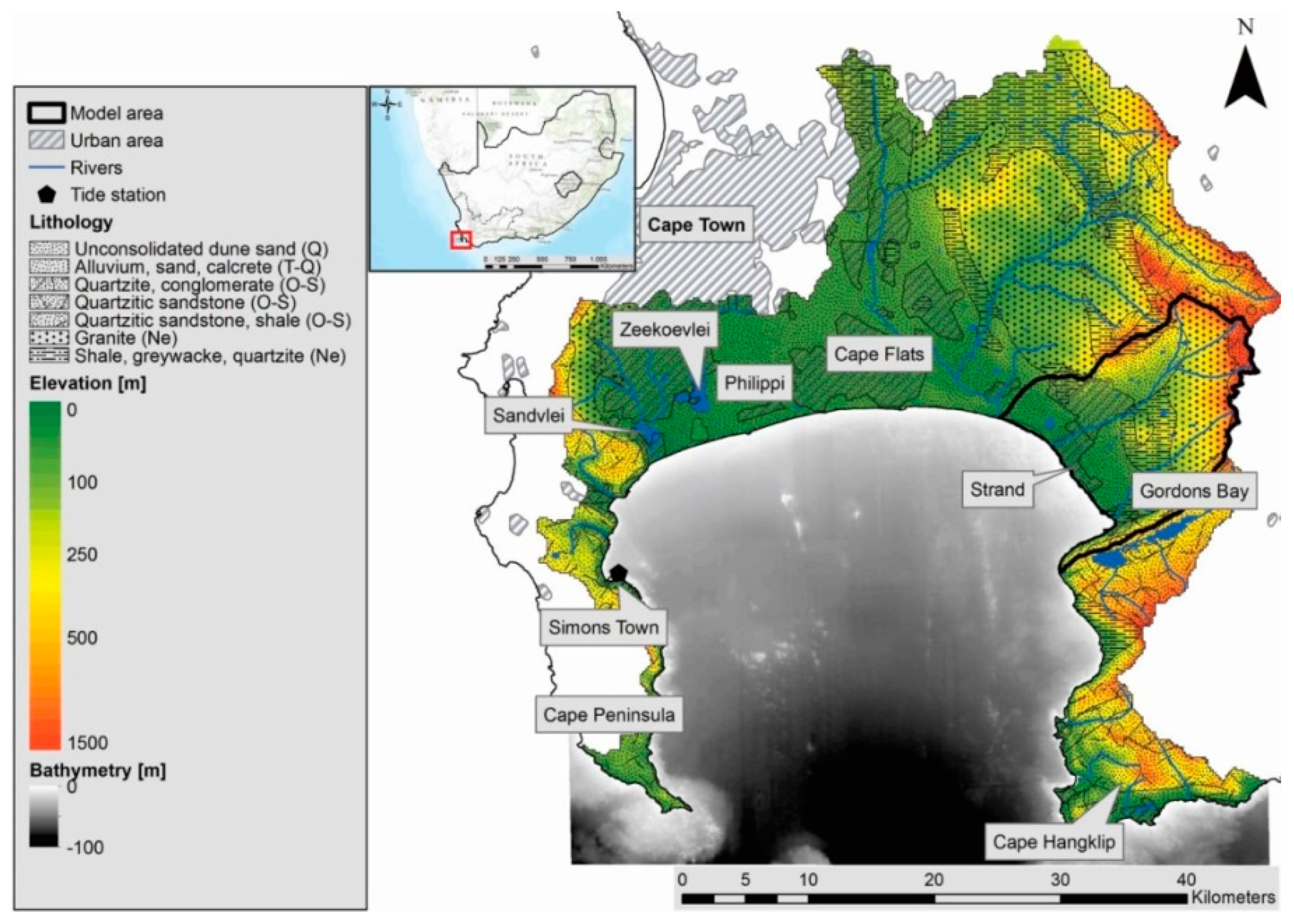
2.1. Study Area
2.2. Methods
2.2.1. Sampling and Analytical Techniques
Radon Mapping and RMB Offshore Endmember Determination
RMB Endmember Determination for Terrestrial Groundwater and Marine Pore Water
223Ra and 224Ra Detection in Groundwater and Seawater
2.2.2. Processing of the Radon Mapping Data
2.2.3. Radon Mass Balance for the AOI
General RBM Setup
Calculation of the Offshore Radon Mixing Loss
Calculation of the Radon Degassing Loss
Calculation of Radon Decay, Production and Diffusive Flux
RMB Endmember Uncertainty Propagation
2.2.4. FSGD/RSGD Differentiation
2.2.5. Validation of the RMB Results Using Hydrogeological and Hydrological Models
3. Results
3.1. SGD Localization
3.1.1. Radon Mapping in the Coastal Sea
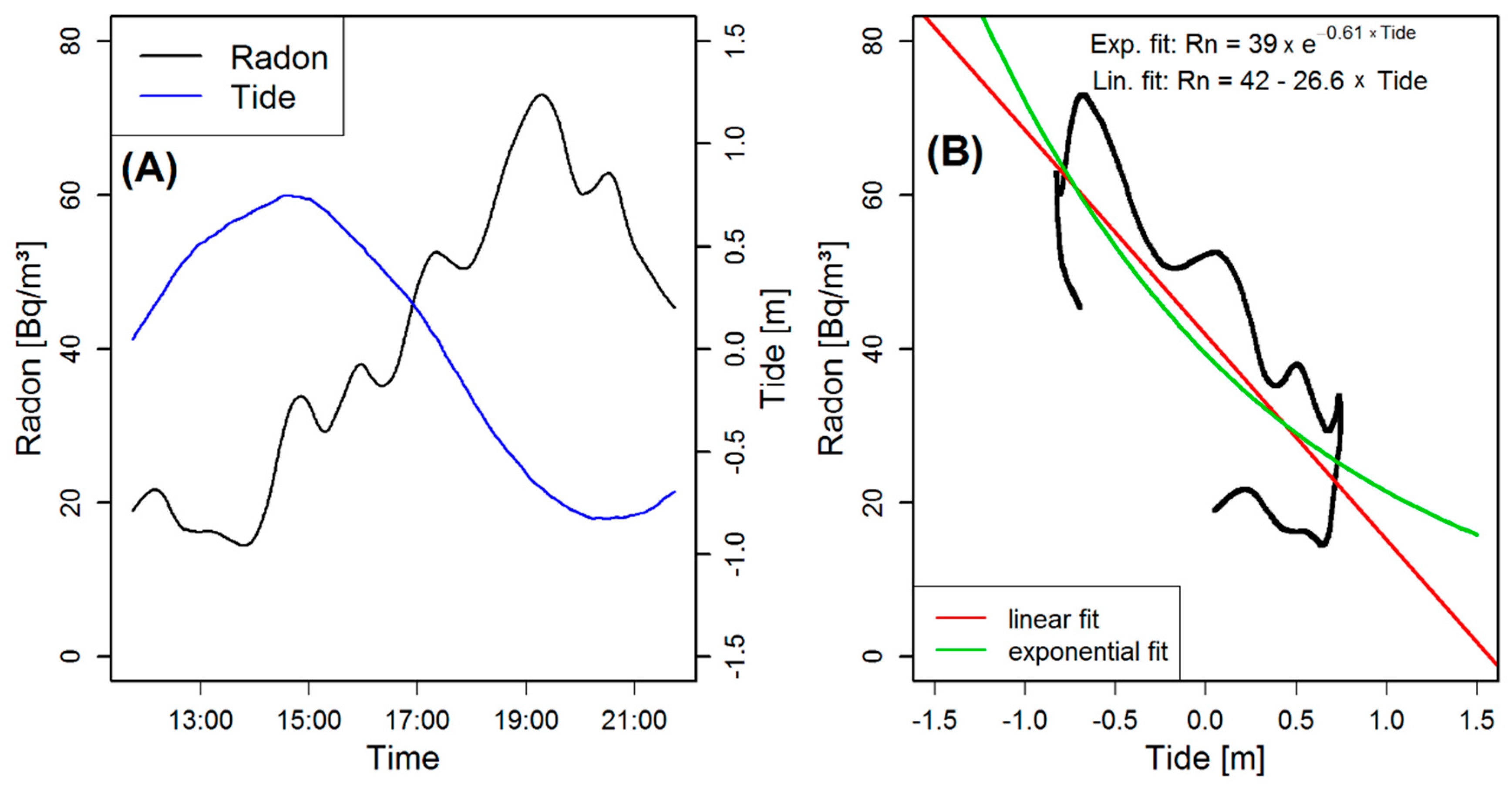
Tide Correction of Radon Time Series
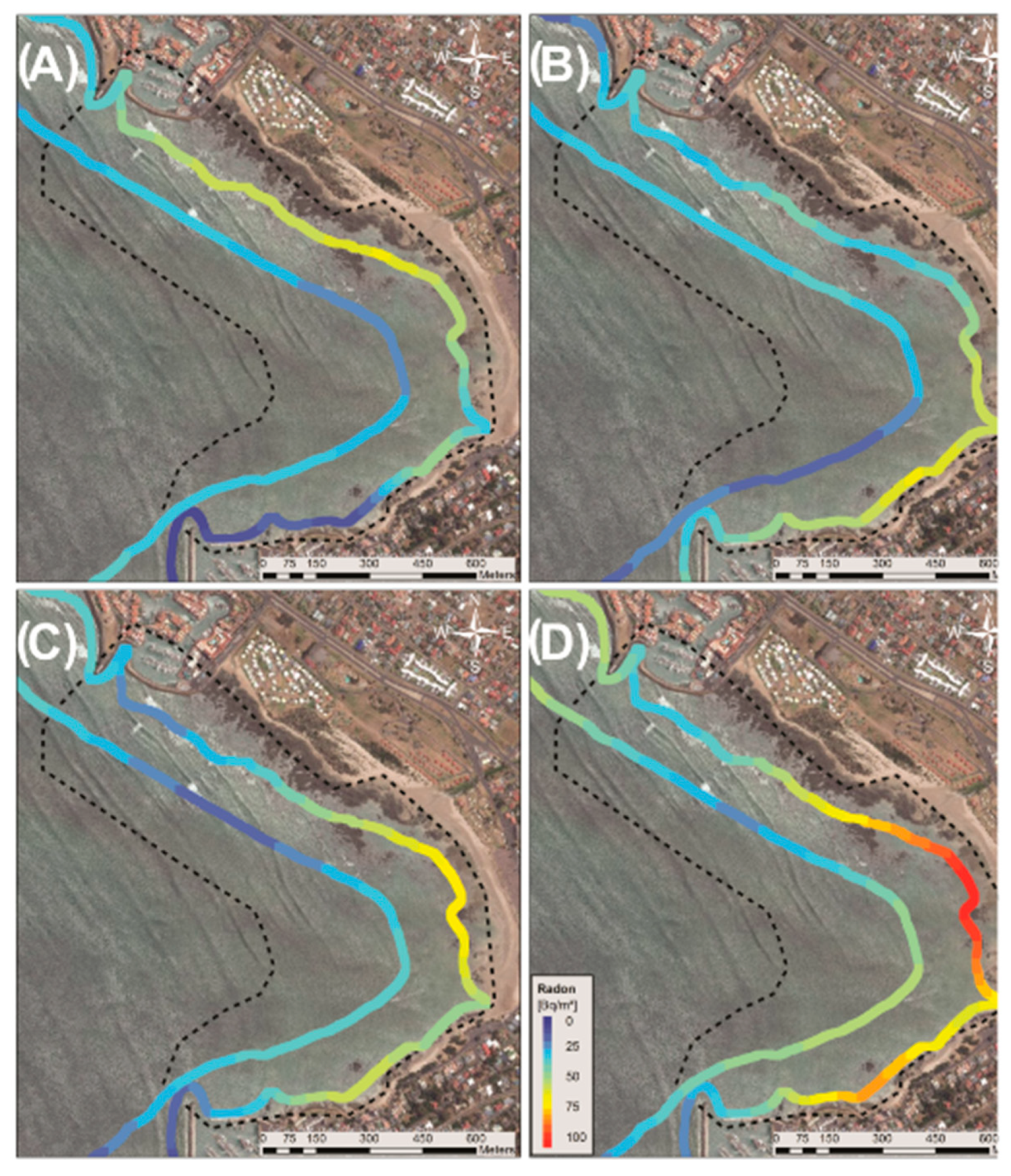
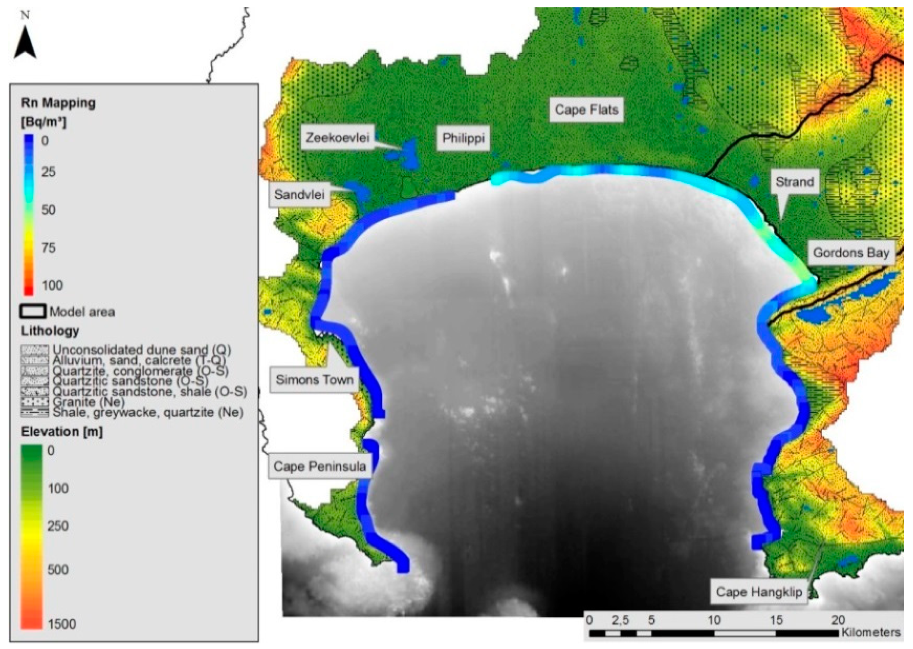
Radon Distribution along the False Bay Coastline
Radon Distribution within the AOI
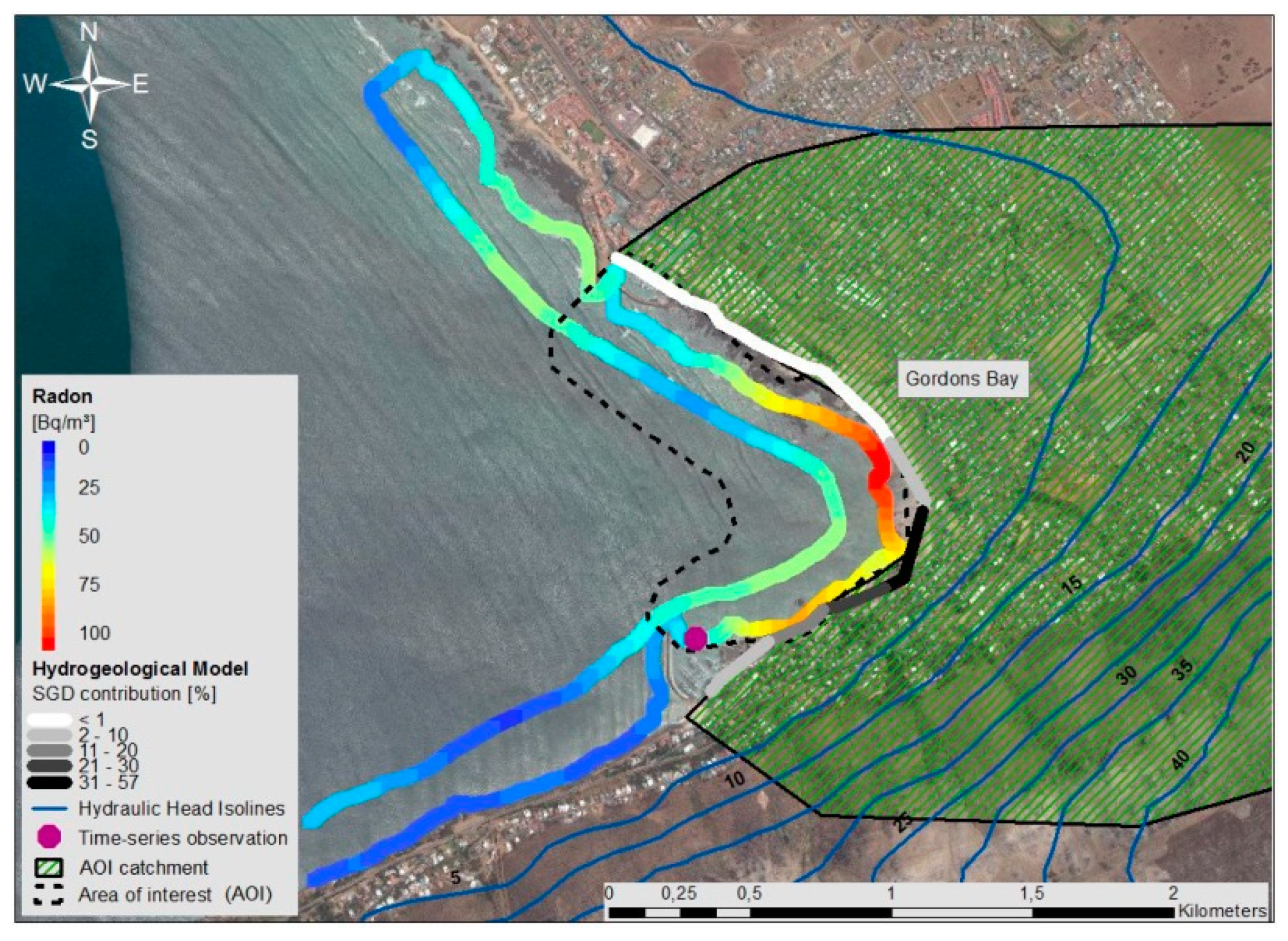
3.1.2. Hydrogeological Modelling
3.2. SGD Quantification within the AOI
3.2.1. Radon Mass Balance
AOI Definition and Radon Inventory Calculation
Calculation of AOI Radon Losses and Radon Inputs
Mixing Loss
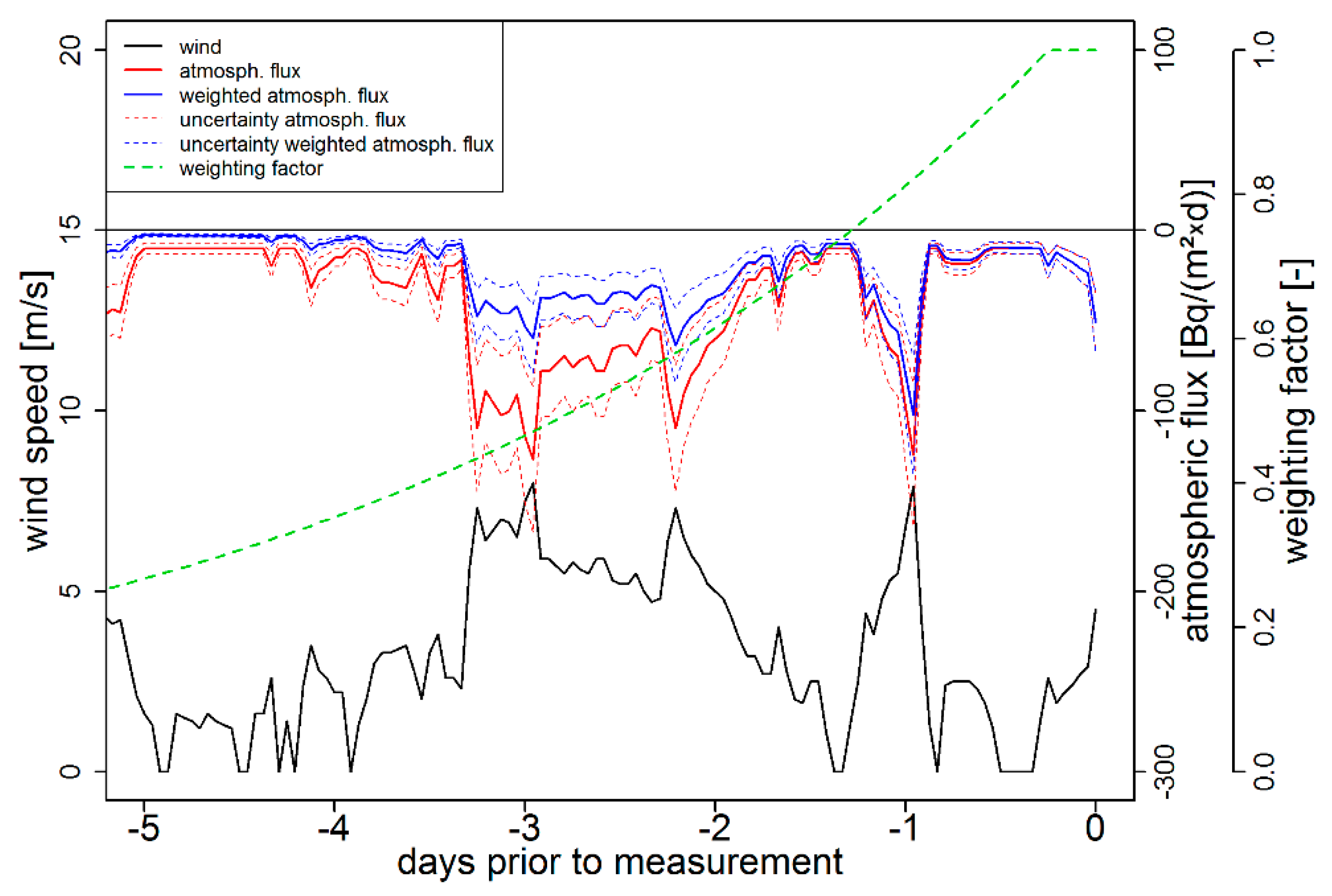
Degassing Loss
Decay Loss
Diffusive Input from Sediment
Input by Seawater in-situ Radon Production
Terrestrial Radon Endmember in Beach Sediment Pore Water
Radon and Water Flux Associated with SGD
3.2.2. Differentiation between FSGD and RSGD
4. Discussion
4.1. Appropriateness of the Introduced Approach
4.2. General SGD Occurance in False Bay
4.3. SGD Quantification for the AOI
5. Conclusions
Author Contributions
Funding
Acknowledgments
Conflicts of Interest
References
- Watson, R.T.; Zakri, A.H. MEA—Millennium Ecosystem Assessment. Ecosystems and Human Well-Being: Synthesis; Island Press: Washington, DC, USA, 2005. [Google Scholar]
- Rasch, P.S.; Ipsen, N.; Malmgren-Hansen, A.; Mogensen, B. Linking integrated water resources management and integrated coastal zone management. Water Sci. Technol. 2005, 51, 221–229. [Google Scholar] [CrossRef] [PubMed]
- Church, T.M. An underground route for the water cycle. Nature 1996, 380, 579–580. [Google Scholar] [CrossRef]
- Moore, W.S. The subterranean estuary: A reaction zone of ground water and sea water. Mar. Chem. 1999, 65, 111–125. [Google Scholar] [CrossRef]
- Moore, W.S. The Effect of Submarine Groundwater Discharge on the Ocean. Ann. Rev. Mar. Sci. 2010, 2, 59–88. [Google Scholar] [CrossRef] [PubMed]
- Campbell, E.E.; Bate, G.C. Tide-induced pulsing of nutrient discharge from an unconfined aquifer into an Anaulis australis-dominated surf zone. Water SA 1998, 24, 365–370. [Google Scholar]
- Hu, C.; Muller-Karges, F.E.; Swarzenski, P.W. Hurricanes, submarine groundwater discharge, and Florida’s red tides. Geophys. Res. Lett. 2006, 33, L11601. [Google Scholar] [CrossRef]
- Laroche, J.; Nuzzi, R.; Waters, R.; Wyman, K.; Falkowski, P.; Wallace, D. Brown Tide blooms in Long Island’s coastal waters linked to interannual variability in groundwater flow. Glob. Chang. Biol. 1997, 3, 397–410. [Google Scholar] [CrossRef]
- Oliveira, J.; Burnett, W.C.; Mazilli, B.P.; Braga, E.S.; Farias, L.A.; Christoff, J.; Furtado, V.V. Reconnaissance of SGD at Ubatuba coast, Brazil, using 222Rn as a natural tracer. J. Environ. Radioact. 2003, 69, 37–52. [Google Scholar] [CrossRef]
- Mejías, M.; Ballesteros, B.; Antón-Pacheco, C.; Domínguez, J.; Garcia-Orellana, J.; Garcia-Solsona, E.; Masqué, P. Methodological study of submarine groundwater discharge from a karstic aquifer in the Western Mediterranean Sea. J. Hydrol. 2012, 464–465, 27–40. [Google Scholar] [CrossRef]
- Wilson, J.; Rocha, C. Regional scale assessment of Submarine Groundwater Discharge in Ireland combining medium resolution satellite imagery and geochemical tracing techniques. Remote Sens. Environ. 2012, 119, 21–34. [Google Scholar] [CrossRef]
- Zekster, I.S.; Loaiciga, A. Groundwater fluxes in the global hydrologic cycle: Past, present and future. J. Hydrol. 1993, 144, 405–427. [Google Scholar] [CrossRef]
- Destouni, G.; Prieto, C. On the possibility for generic modeling of submarine groundwater discharge. Biogeochemistry 2003, 66, 171–186. [Google Scholar] [CrossRef]
- Robinson, C.; Li, L.; Prommer, H. Tide-induced recirculation across the aquifer-ocean interface. Water Resour. Res. 2007, 43, W07428. [Google Scholar] [CrossRef]
- Li, X.; Hu, B.; Burnett, W.C.; Santos, I.; Chanton, J. Submarine Ground Water Discharge Driven by Tidal Pumping in a Heterogenous Aquifer. Ground Water 2009, 47, 558–568. [Google Scholar] [CrossRef]
- Burnett, W.C.; Dulaiova, H. Estimating the dynamics of groundwater input into the coastal zone via continuous radon-222 measurements. J. Environ. Radioact. 2003, 69, 21–35. [Google Scholar] [CrossRef]
- Burnett, W.C.; Dulaiova, H. Radon as a tracer of submarine groundwater discharge into a boat basin in Donnalucata, Sicily. Cont. Shelf Res. 2006, 26, 862–873. [Google Scholar] [CrossRef]
- Stieglitz, T. Submarine groundwater discharge into the near-shore zone of the Great Barrier Reef, Australia. Mar. Pollut. Bull. 2005, 51, 51–59. [Google Scholar] [CrossRef]
- Moore, W.S.; Sarmiento, J.L.; Key, R.M. Submarine groundwater discharge revealed by 228Ra distribution in the upper Atlantic Ocean. Nat. Geosci. 2008, 1, 309–311. [Google Scholar] [CrossRef]
- Schubert, M.; Knoeller, K.; Einsiedl, F.; Rocha, C. Preliminary Evaluation of groundwater contributions to the water budget of Kinvarra Bay, Ireland, using 222Rn, EC and stable isotopes as natural indicators. Environ. Monit. Assess. 2015, 187, 4274. [Google Scholar] [CrossRef]
- Burnett, W.C.; Bokuniewicz, H.; Huettel, M.; Moore, W.S.; Taniguchi, M. Groundwater and pore water inputs to the coastal zone. Biogeochemist 2003, 66, 3–33. [Google Scholar] [CrossRef]
- Wu, Z.; Zhou, H.; Zhang, S.; Liu, Y. Using 222Rn to estimate submarine groundwater discharge (SGD) and the associated nutrient fluxes into Xiangshan Bay, East China Sea. Mar. Pollut. Bull. 2013, 73, 183–191. [Google Scholar] [CrossRef] [PubMed]
- MacIntyre, S.; Wanninkhof, R.; Chanton, J.P. Trace gas exchange across the air–water interface in freshwater and coastal marine environments. In Biogenic Trace Gases: Measuring Emissions from Soil and Water; Matson, P.A., Hariss, R.C., Eds.; Blackwell Science: Hoboken, NJ, USA, 1995; pp. 52–97. [Google Scholar]
- Wen, T.; Du, J.; Ji, T.; Wang, X.; Deng, B. Use of 222Rn to trace submarine groundwater discharge in a tidal period along the coast of Xiangshan, Zhejiang, China. J. Radioanal. Nucl. Chem. 2014, 299, 53–60. [Google Scholar] [CrossRef]
- Santos, I.R.; Eyre, B.D.; Huettel, M. The driving forces of pore water and groundwater flow in permeable coastal sediments: A review. Estuar. Coast. Shelf 2012, 98, 1–15. [Google Scholar] [CrossRef]
- Mulligan, A.; Charette, M. Intercomparison of submarine groundwater discharge estimates from a sandy unconfined aquifer. J. Hydrol. 2006, 327, 411–425. [Google Scholar] [CrossRef]
- McCoy, C.A.; Corbett, D.R. Review of submarine groundwater discharge (SGD) in coastal zones of the Southeast and Gulf Coast regions of the United States with management implications. J. Environ. Manag. 2009, 90, 644–651. [Google Scholar] [CrossRef] [PubMed]
- Petermann, E.; Schubert, M. Quantification of the response delay of mobile Rn-in-air detectors applied for detecting short-term fluctuations of Rn-in-water concentrations. Eur. Phys. J. Spec. Top. 2015, 224, 697–707. [Google Scholar] [CrossRef]
- IAEA The GNIP Database. Station 6881600 ‘Malan’ (Cape Town) South Africa. Global Network of Isotopes in Precipitation. Available online: https://www.iaea.org/services/networks/gnip (accessed on 5 April 2019).
- Adelana, S.; Xu, Y.; Vrbka, P. A conceptual model for the development and management of the Cape Flats aquifer, South Africa. S. Afr. Water Res. Comm. 2010, 36. [Google Scholar] [CrossRef]
- Meyer, P.S. An Explanation of the 1:500000 General Hydrogeological Map Cape Town 3317; Department of Water Affairs and Forestry: Cape Town, South Africa, 2001.
- Haskins, C. False Bay Ecology Park Water Quality Report; Transport for Cape Town Planning Department: Cape Town, South Africa, 2015.
- Van Niekerk, A. Stellenbosch University Digital Elevation Model (SUDEM)—2013 Edition, Product Description; Centre for Geographical Analysis, Stellenbosch University: Stellenbosch, South Africa, 2013; p. 15. [Google Scholar]
- Schmidt, A.; Schlüter, M.; Melles, M.; Schubert, M. Continuous and discrete on-site detection of radon-222 in ground- and surface waters by means of an extraction module. Appl. Radiat. Isot. 2008, 66, 1939–1944. [Google Scholar] [CrossRef]
- Schubert, M.; Paschke, A.; Lieberman, E.; Burnett, W.C. Air−Water Partitioning of 222Rn and its Dependence on Water Temperature and Salinity. Environ. Sci. Technol. 2012, 46, 3905–3911. [Google Scholar] [CrossRef]
- Schubert, M.; Bürkin, W.; Peña, P.; Lopez, A.; Balcázar, M. On-site determination of the Rn concentration in water samples: Methodical background and results from laboratory studies and a field-scale test. Radiat. Meas. 2006, 41, 492–497. [Google Scholar] [CrossRef]
- Bourquin, M.; van Beek, P.; Reyss, J.L.; Souhaut, M.; Charette, M.A.; Jeandel, C. Comparison of techniques for pre-concentrating radium from seawater. Mar. Chem. 2008, 109, 226. [Google Scholar] [CrossRef]
- Moore, W.S.; Arnold, R. Measurement of 223Ra and 224Ra in coastal waters using a delayed coincidence counter. J. Geophys. Res. 1996, 101, 1321–1329. [Google Scholar] [CrossRef]
- Scholten, J.C.; Pham, M.K.; Blinova, O.; Charette, M.A.; Dulaiova, H.; Eriksson, M. Preparation of Mn-fiber standards for the efficiency calibration of the delayed coincidence counting system (RaDeCC). Mar. Chem. 2010, 121, 206–214. [Google Scholar] [CrossRef]
- Moore, W.S.; Cai, P. Calibration of RaDeCC systems for 223Ra measurements. Mar. Chem. 2013, 156, 130–137. [Google Scholar] [CrossRef]
- Garcia-Solsona, E.; Garcia-Orellana, J.; Masqué, P.; Dulaiova, H. Uncertainties associated with 223Ra and 224Ra measurements in water via a Delayed Coincidence Counter (RaDeCC). Mar. Chem. 2008, 109, 198–219. [Google Scholar] [CrossRef]
- Dimova, N.T.; Burnett, W.C. Evaluation of groundwater discharge into small lakes based on the temporal distribution of Rn-222. Limnol. Oceanogr. 2011, 56, 486–494. [Google Scholar] [CrossRef]
- Burnett, W.C.; Peterson, R.; Moore, W.S.; Oliveira, J. Radon and radium isotopes as tracers of submarine groundwater discharge e Results from the Ubatuba, Brazil SGD assessment intercomparison. Estuar. Coast. Shelf Sci. 2008, 76, 501–511. [Google Scholar] [CrossRef]
- Moore, W.S. Radium isotopes as tracers of submarine groundwater discharge in Sicily. Cont. Shelf Res. 2006, 26, 852–861. [Google Scholar] [CrossRef]
- Martens, C.; Kipphuit, W.; val Klump, J. Sediment-Water Chemical Exchange in the Coastal Zone Traced by in situ Rn-222 Flux Measurements. Science 1980, 208, 285–288. [Google Scholar] [CrossRef]
- Lambert, M.; Burnett, W.C. Submarine groundwater discharge estimates at a Florida coastal site based on continuous radon measurements. Biogeochemistry 2003, 66, 55–73. [Google Scholar] [CrossRef]
- Zikovsky, L.; Chah, B. The lognormal distribution of radon concentration in ground water. Ground Water 1990, 28, 673–676. [Google Scholar] [CrossRef]
- Department of Water Affairs and Forestry. Task 1BC—Groundwater Quantification. Methodology Report. In Groundwater Resource Assessment; Department of Water Affairs and Forestry: Cape Town, South Africa, 2004; p. 41. [Google Scholar]
- Gebel, M.; Halbfaß, S.; Bürger, S.; Lorz, C. Long-term simulation of effects of energy crop cultivation on nitrogen leaching and surface water quality in Saxony/Germany. Reg. Environ. Chang. 2012, 2012. [Google Scholar] [CrossRef]
- Gebel, M.; Meißner, R.; Halbfaß, S.; Hagenau, J.; Duan, S. Web GIS-based simulation of water fluxes in the Miyun catchment area. iForest 2014, 2014, 363. [Google Scholar] [CrossRef]
- Gebel, M.; Bürger, S.; Wallace, M.; Malherbe, H.; Vogt, H.; Lorz, C. Simulation of land use impacts on sediment and nutrient transfer in coastal areas of Western Cape, South Africa. Chang. Adapt. Socioecol. Syst. 2017, 3, 1–17. [Google Scholar] [CrossRef]
- Allen, R.G.; Pereira, L.S.; Raes, D.; Smith, M. Crop Evapotranspiration—Guidelines for computing crop water requirements. FAO Irrig. Drain. Pap. 1998, 56. Available online: www.researchgate.net/publication/284300773_FAO_Irrigation_and_drainage_paper_No_56 (accessed on 5 April 2019).
- Hawkins, R.H.; Ward, T.J.; Woodward, D.E.; Van Mullem, J.A. Curve Number Hydrology: State of the Practice; American Society of Civil Engineers: Reston, VA, USA, 2009. [Google Scholar]
- NRCS. National Engineering Handbook Part 630 Hydrology—Estimation of Direct Runoff from Storm Rainfall; United States Department of Agriculture, Natural Resources Conservation Service: Washington, DC, USA, 2004. [Google Scholar]
- Michael, H.; Mulligan, A.; Harvey, C. Seasonal oscillations in water exchange between aquifers and the coastal ocean. Nat. Lett. 2005, 436, 1145–1148. [Google Scholar] [CrossRef]


© 2019 by the authors. Licensee MDPI, Basel, Switzerland. This article is an open access article distributed under the terms and conditions of the Creative Commons Attribution (CC BY) license (http://creativecommons.org/licenses/by/4.0/).
Share and Cite
Schubert, M.; Petermann, E.; Stollberg, R.; Gebel, M.; Scholten, J.; Knöller, K.; Lorz, C.; Glück, F.; Riemann, K.; Weiß, H. Improved Approach for the Investigation of Submarine Groundwater Discharge by Means of Radon Mapping and Radon Mass Balancing. Water 2019, 11, 749. https://doi.org/10.3390/w11040749
Schubert M, Petermann E, Stollberg R, Gebel M, Scholten J, Knöller K, Lorz C, Glück F, Riemann K, Weiß H. Improved Approach for the Investigation of Submarine Groundwater Discharge by Means of Radon Mapping and Radon Mass Balancing. Water. 2019; 11(4):749. https://doi.org/10.3390/w11040749
Chicago/Turabian StyleSchubert, Michael, Eric Petermann, Reiner Stollberg, Micha Gebel, Jan Scholten, Kay Knöller, Carsten Lorz, Franziska Glück, Kornelius Riemann, and Holger Weiß. 2019. "Improved Approach for the Investigation of Submarine Groundwater Discharge by Means of Radon Mapping and Radon Mass Balancing" Water 11, no. 4: 749. https://doi.org/10.3390/w11040749