Study on the Assessment Method of the Impact on Hydrological Safety of Riverside Pit-Ponds along a Dike
by
Shuai Liu
1,2, 
Dewei Yang
2,3,*,
Jinbao Sheng
2,3,
Jiankang Chen
1,
Chengjun Xu
4 and
Yingying Chen
2 1
State Key Laboratory of Hydraulics and Mountain River Engineering, College of Water Resource and Hydropower, Sichuan University, Chengdu 610065, China
2
Nanjing Hydraulic Research Institute, Nanjing 210029, China
3
Dam Safety Management Center of the Ministry of Water Resources, Nanjing 210029, China
4
Jiangsu Kexing Project Management Co., Ltd., Nanjing 210029, China
*
Author to whom correspondence should be addressed.
Water 2019, 11(4), 744; https://doi.org/10.3390/w11040744
Submission received: 7 March 2019
/
Revised: 27 March 2019
/
Accepted: 6 April 2019
/
Published: 10 April 2019
(This article belongs to the Section Water Resources Management, Policy and Governance)
Abstract
:Riverside pit-ponds are one of the hidden dangers of flood control project safety. At present, the safety evaluation of riverside pit-ponds is limited to the seepage and stable safety review of the dam, and the impact of the pit on the river flow is not considered. In this paper, a two-dimensional mathematical model of flow is established. Pressure correction method is used to solve the pressure-velocity coupling. Topographic cutting method is used to deal with the dynamic boundary problem. The model grid of the pit-ponds area is encrypted. The accuracy of the model in the analysis of river hydrodynamics is verified by an example. The model is applied to the evaluation of the impact of the pit-ponds on river flooding. Taking some riverside pit-ponds of the Yellow River as an example, the river water level, velocity, and flow in the present condition and the backfill condition are simulated by the model. The results show that the existence of these riverside pit-ponds only affects the hydrological features of regions around the pit-ponds, and the impact is too insignificant to threaten the hydrological safety. Through the hydrological safety assessment of the project, it is shown that the combination of the two-dimensional flow mathematical model with seepage, anti-sliding, and seismic safety review can comprehensively assess the hydrological safety of dike engineering.
1. Introduction
As the oldest and most basic flood control facilities, dike projects are widely used in China. At present, the length of the dike project built in China is nearly 420,000 km [1]. According to relevant statistics [2], almost half of China’s population, and one-third of the arable land and two-thirds of the gross industrial and agricultural product are under the protection of dikes. Thus, it can be seen that the flood control safety of the dike project is of great importance. There are many factors that affect the flood control safety of the dike project, with near dike pit-ponds being one of them.
Due to flood erosion, earth borrowing for the construction of dikes, and earth borrowing for housing, some pit-ponds are left behind on the riverside of the dike, most of which accumulate water all year round and have been used as fish ponds for fish farming. In the Pearl River Delta region, a well-developed pond ecosystem has been formed [3,4]. However, the existence of riverside pit-ponds has always been a safety hazard for dike flood control, because it has changed the ground elevation on both sides of the dike, reduced the stability of the dike, and destroyed the impermeable water layer or weak water layer of the original surface [5], causing changes in the seepage field of the dam. In actual projects, the pit-ponds filling method is often used to deal with these pit-ponds [6]. However, it is relatively reasonable to choose the dangerous pit-ponds for filling through the safety evaluation of pit-ponds. In the past, only the impact of the pit-ponds on the seepage and slope stability of the dike was considered for the safety evaluation of the pit-ponds [5], and the impact of the pit-ponds on the flood flow of the river was not considered, which is not perfect. The existence of pit-ponds is bound to affect hydrologic factors, such as water level, flow velocity, and flow volume during floods. Therefore, it is of great significance to break through the traditional evaluation method on the problem that riverside pit-ponds affecting flood control safety.
In recent decades, the development of computers and the improvement of computing technology have provided conditions for the use of mathematical models to study the movement of water flow. Among them, due to the reliable results and simple calculation, the two-dimensional water flow mathematical model is widely used in water network simulation [7,8], river regulation [9], sediment transport [10,11], flood prediction [12,13], dike engineering [14,15], and other aspects. In 1992, the two-dimensional finite element method was adopted by Bates PD [16] to simulate the floodplain flow, laying a foundation for floodplain simulation. Domestically, Sun Dongpo et al. [15] first applied the two-dimensional water flow mathematical model to the analysis and evaluation of the impact of the production dikes on floods, and typical flood simulation was carried out for three conditions of the Yellow River, such as producing dikes, abolishing production dikes, and limiting production dikes. Xu Hui et al. [17] proposed a new method for numerical simulation of two-dimensional water flow in a submerged spur dam group using a new grid node arrangement and established a mathematical model. The simulation results were consistent with the measured results. Shi Yingbiao [12] creatively introduce the irregular triangular mesh into the two-dimensional flow mathematical model of water and sand transportation in complex rivers, and the disadvantages of the poor adaptability of structural rectangular grid to irregular coastline and complex terrain in natural rivers was improved.
The two-dimensional water flow mathematical model is applied in this paper for evaluating the safety of pit-ponds, with the pit-ponds on the riverside of a section of the Yellow River being cited as examples, the current conditions and the backfilling conditions of the pit-ponds are simulated, and the influence of the pit-ponds on the flood flow of the river is analyzed. Concurrently, combined with seepage, anti-sliding, and a seismic resistance safety review of the dam, the flood control safety of the dike project is comprehensively evaluated, thus providing a new idea for the safety evaluation and handling of similar projects.
2. Establishment of a Two-Dimensional Mathematical Model of Water Flow
2.1. Control Equation
Continuous equation:
Momentum equation:
where: , are components of the depth-averaged components of water flow velocity in the x- and y-direction; h is the water depth below the water surface; is the water level fluctuation, ; is the Coriolis force coefficient, , is the earth’s angular velocity, is the latitude, is the effective viscosity coefficient, is the kinematic viscosity coefficient, is the turbulent viscosity coefficient, ; are components of the bottom shear stress in the x- and y-direction of , , respectively, is the bottom friction coefficient; are components of the surface wind stress in the x- and y-direction. This model does not consider the influence of wind stress for the moment, and lets be zero.
The above governing equations can be written as a unified convection-diffusion differential equation:
where the calculated variable is , is source item. By negatively ramping the source term linearly: , must be met; ; , is the empirical constant.
2.2. Discrete Solution of Equations
Using coordinate transformation, the Cartesian coordinate system pair of convection-diffusion differential Equation (4) can be transformed into the (ξ, η) plane unified convection-diffusion differential equation:
where , , U, V are inverse speed flux components in the corresponding (ξ, η) coordinate system; J is diffusion flux; , , .
The differential equations are discrete as follows:
where , , , ;
The pressure correction method is used for coupling the pressure-flow rate. The main steps are as follows:
(1) Given the initial water level prediction value ;
(2) The momentum equation is solved with the corresponding , while the velocity equation of U* and V* may not be necessarily satisfied.
(3) The flow rate fluxes , of the control volume interface are calculated by the momentum interpolation calculation formula.
(4) The water level correction equation is solved and is obtained.
(5) The corrected water level is solved by the SIMPLE method, and the SIMPLEC method is used to correct the flow velocity to obtain U and V.
(6) With the corrected water level ζ as the new predicted water level , return to the second step and repeat the whole process until a convergent solution is obtained.
2.3. Boundary Conditions
In the two-dimensional flow digital model, the boundary conditions usually include the bank boundary, the inlet boundary, the exit boundary, and the dynamic boundary. The model adopts the following boundary conditions.
(1) Initial conditions:
Given the initial condition at moment t = 0, the initial value of all computational variables (U, V, ζ, K, ε, Si, Ni) in the domain can be obtained (U0, V0, ζ0, Kε0, Si0, Ni0).
(2) Control boundary conditions:
Upstream import conditions: The upstream section uses the flow process line, and the flow velocity of each control point is calculated by the following formula:
where Uj, hj is flow point and water depth of the calculated grid point along the y direction, is discrete grid spacing.
Vj = 0, the turbulent kinetic energy of , is a constant, turbulent dissipation rate of , and B is the width of the river.
Given the water level control of and , the flow velocity of at import points, the turbulent kinetic energy and turbulent dissipation rate are calculated as above.
(3) Solid wall conditions:
The flow velocity uses no sliding boundary conditions, U = V = 0. Due to the turbulent energy dissipation on the solid wall boundary, in the model, the solid wall conditions are to be specially treated, and the near-shore flow rate Uτ satisfies the logarithmic flow rate distribution relationship:
where , is shore wall resistance velocity; is the distance between the grid point and the shore wall; E is the parameter that represents the roughness rate; k is the Carmen’s constant.
(4) Convergence control condition:
Control the maximum mass source of the continuous equation, though the flow Qj of each section, ; flow velocity m/s; water level m.
2.4. Parameter Selection and Boundary Simulation
(1) Selection of calculation parameters
The mathematical model calculation involves the selection of many calculation parameters. The selection of calculation parameters, such as roughness coefficient, turbulent viscosity coefficient, and calculation step length in the two-dimensional flow mathematical model affect the calculation process and calculation results. The average flow velocity of the natural river channel is related to the hydraulic radius, river ratio drop, and roughness coefficient. It is somewhat similar to the ground friction coefficient. The lower the roughness, the higher the flow rate. The determined roughness factor is, therefore, a defined value for determining the flow rate and other relevant parameters. Therefore, the value of roughness coefficient n in the calculation process is: Main channel, , floodplain . Termination of the turbulent viscosity coefficient of the water flow is based on the zero-equation turbulent model, , where is the friction flow rate, α is constant, and generally α is 1–10. This paper calculates the step length as Δt = 10–30 s.
(2) Dynamic boundary simulation
The terrain cutting method is used to deal with dynamic boundary problems, which can easily solve the calculation of irregular open beach and avoid the unstable factors caused by the handling of moving boundary conditions. From the moment of tn to tn + k = tn + kΔt (k ≥ 1), for node i, the depth of : (1) If (dh is the critical depth of the exposed beach), that is, a computable node that does not need to be processed. (2) If , the node is an exposed beach, so it needs to be processed to temporarily reduce the terrain of the node, so that the depth of node is calculated as dh, while taking the larger roughness coefficient and viscosity coefficient. Once the actual water depth is judged to be greater than the critical water depth of the exposed beach, the original terrain will be restored in time.
3. Model Verification
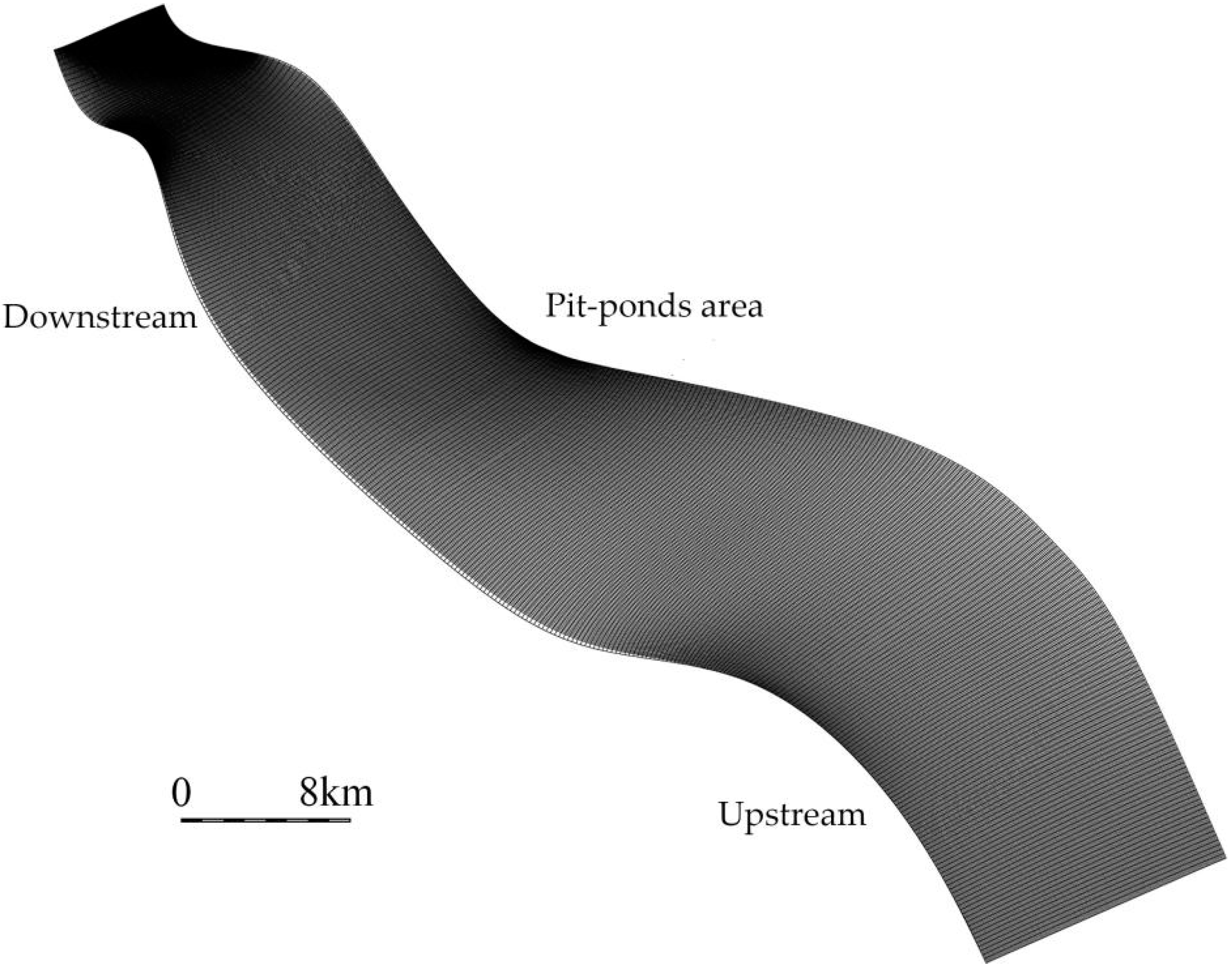
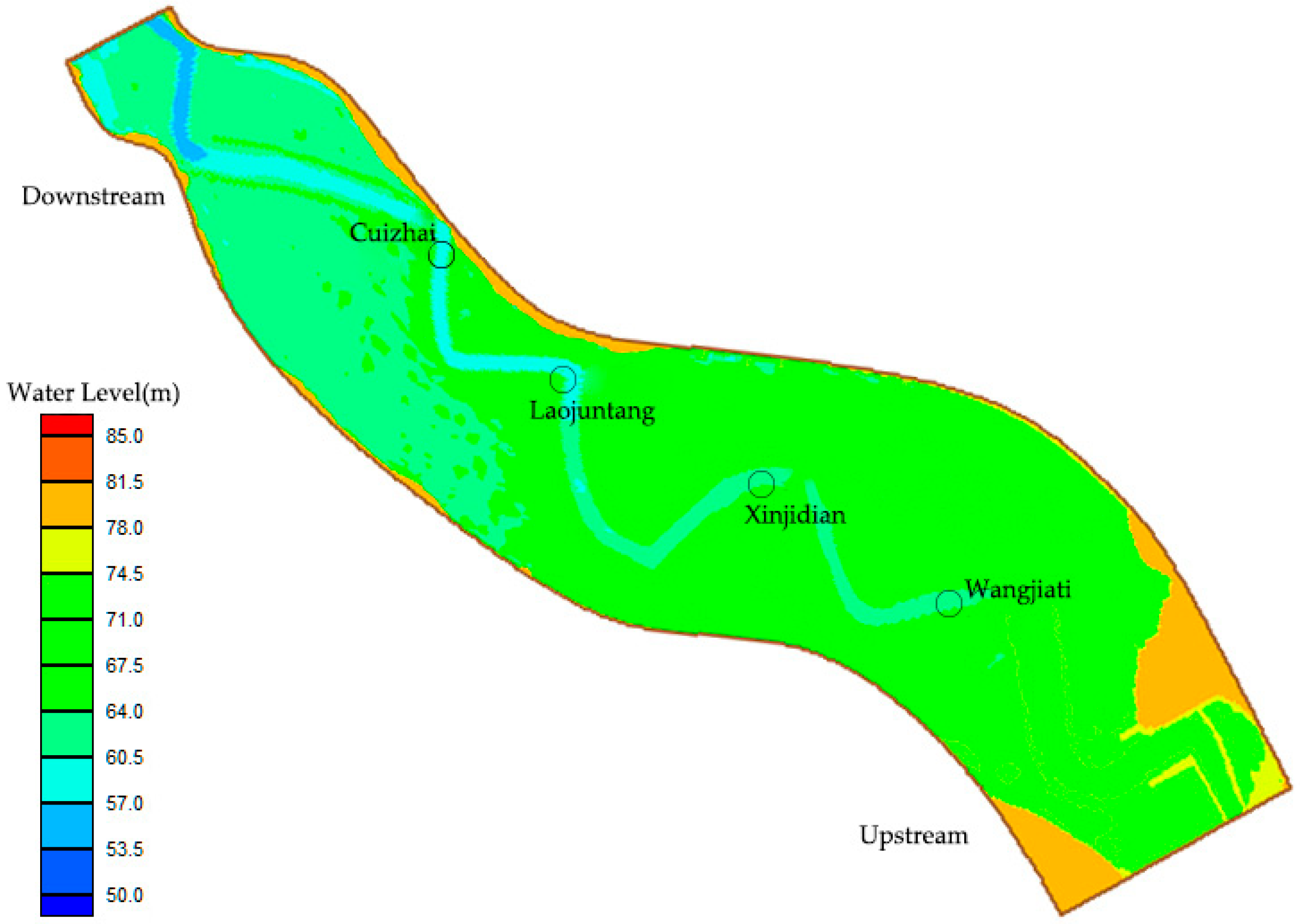
Taking consideration of the calculation scope, import and export conditions, hydrological data, and the scope of the project, a section of the Yellow River with a total length of about 70 km is selected for model accuracy verification. The computational space step length of the verification model is from 15 to 300 m, with a total of approximately 71,757 grid nodes, 59,800 units, and the minimum spacing is approximately 15 m, which fully reflects the dike production, flood protection dams, and the topography of the pit-ponds. The side length of this mesh is the space step length and the minimum spacing is the minimum value for mesh spacing. The grid of the model river section is shown in Figure 1, and the channel bathymetry after grid generation is shown in Figure 2. The discrete terrain basically reflects the measured terrain of the engineering river section.
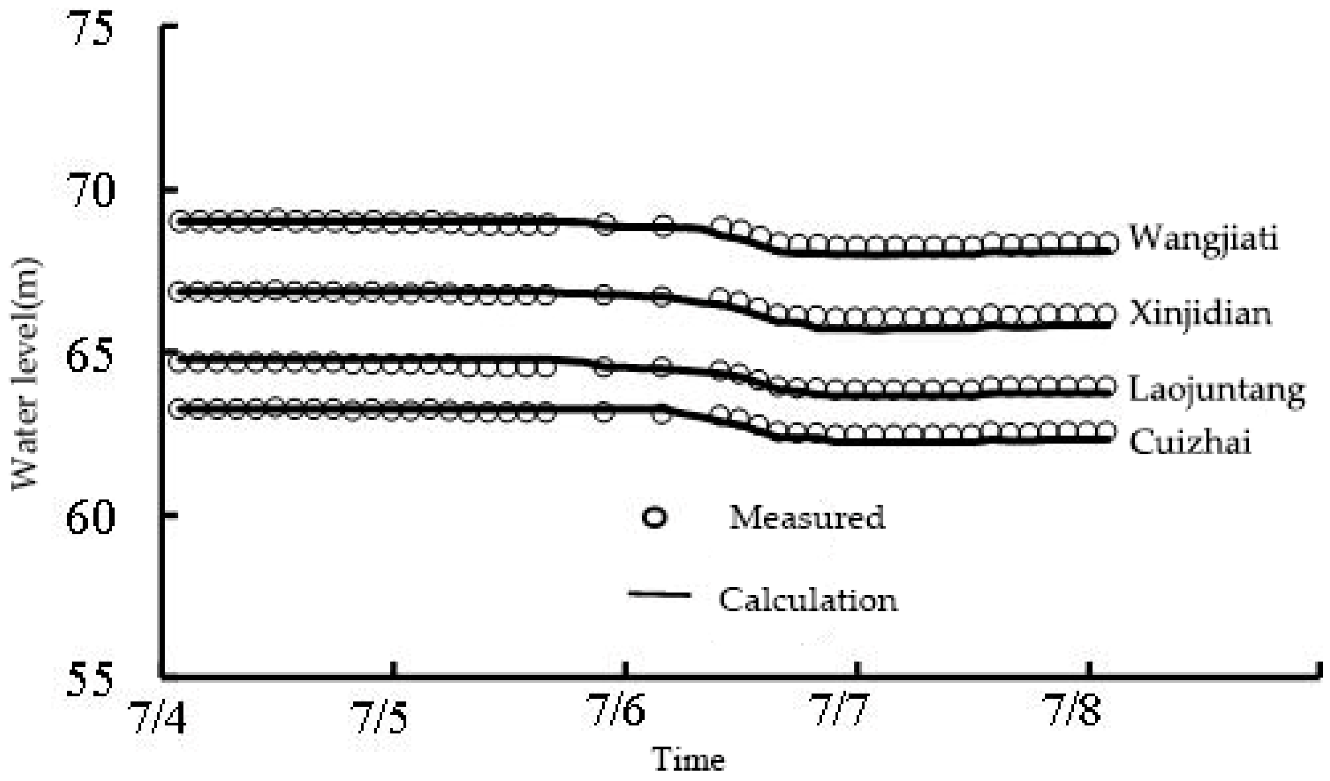
The measured water level data for the four Hydrographic stations in July 2014 are used to verify hydrological data. In the process of verification and calculation, the flow hydrograph is used in the upstream section and the water stage hydrograph is used in the downstream section as the boundary condition. The calculation time step takes s; the critical depth dh of the exposed beach takes 0.1 m. The relevant calculation parameters, such as roughness coefficient, turbulence viscosity coefficient, and length of calculation time, are determined by rate determination; the results are shown in Figure 3. It can be seen from the figure that the calculated value is basically in agreement with the measured water level process, and the error meets the requirements of the specification. It can be seen that the model calculation better simulates the process of water level change along the course, reflecting the comprehensive resistance effect of the river channel.
4. Case Analysis
The length of the section of the Yellow River is about 76 km, the distance between the two banks of the river is 4.1 to 20 km, and the height of the dike is 8 to 12 m. The soil layer can be divided into four layers from top to bottom: artificial filled soils, low liquid limit clay, low liquid limit powdery clay, and low liquid limit clay. In the process of rehabilitation of the Yellow River dike, there are 16 pit-ponds in the riverside of the Yellow River due to the digging earth in the neighborhood, among other reasons, which are distributed within 100 to 650 m from the foot of the dike, with an average depth of 8 m and an area of 10,000 m2 to 100,000 m2. The flood control standard of this section is set based on the upstream control section of 2200 m3/s flow leakage flood fortification. In order to ensure the stability of the Yellow River and the safety of the Yellow River dike, it is necessary to study the impact of the riverside pit-ponds under the floodplain conditions and the safety of the dike, so as to provide scientific basis for the safe operation and management of the dike.
4.1. Hydrodynamic Analysis of the Pit-Ponds Section
The two-dimensional flow model is used to calculate and compare the changes of flood water level, flow velocity, and cross-section flow under the two conditions of current terrain and pit backfilling. According to the engineering situation, five computational operating conditions are selected, that is, upstream import flow Q = 4000 m3/s (local burst floodplain), Q = 7000 m3/s (floodplain), Q = 10,000 m3/s (floodplain), Q = 15,000 m3/s (floodplain), Q = 22,000 m3/s (floodplain). Q is discharge.
4.1.1. Influence of Backfilling in Pit-Ponds on Water Level
In order to analyze the impact of pit-pond backfilling on the water level, 27 water level measuring points are selected along the main channel and on both sides. The water level changes before and after the project are shown in Figure 4. It can be seen that there is almost no change in the water level before and after the project under various hydrological conditions. Under the condition of Q = 22,000 m3/s floodplain, the maximum water damming height in the pit-ponds area is less than 0.03 m, indicating that the backfilling of the pit-ponds has less effect on the flood level of the river.
4.1.2. Influence of Backfilling on Pit Flow Rate
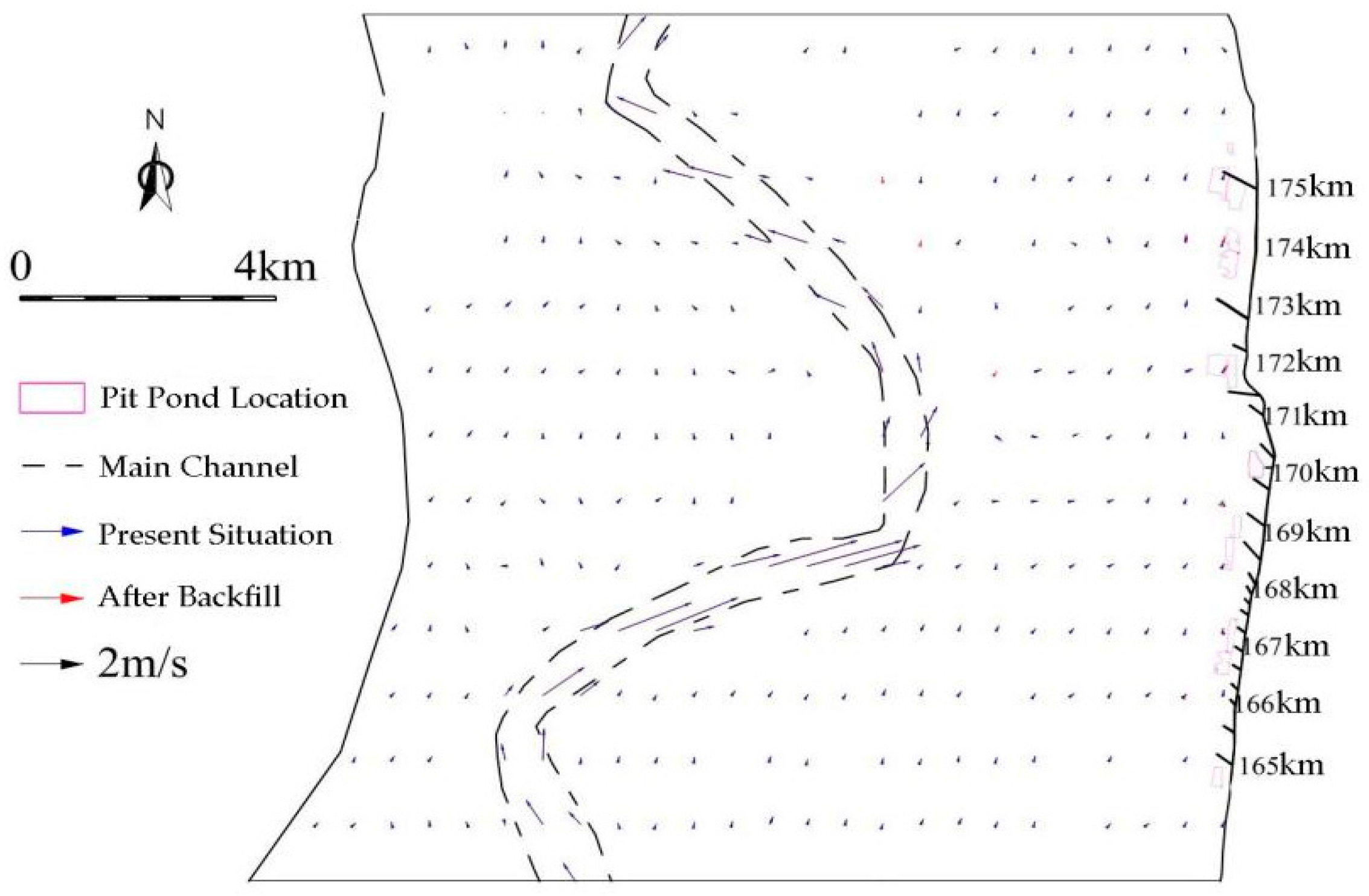
(1) Changes in the flow field
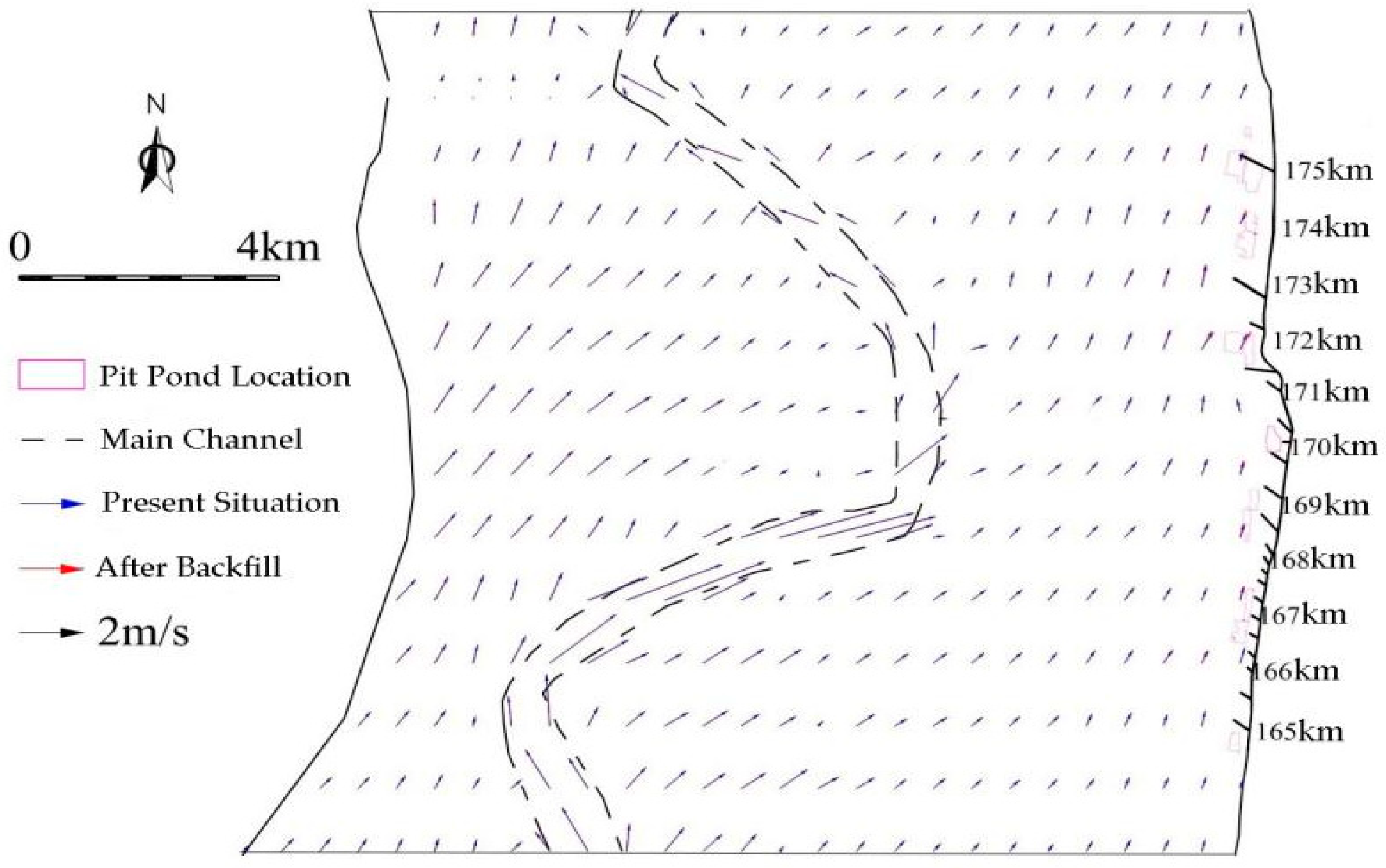
At Q = 7000 m3/s and 22,000 m3/s flow, the flow field under flood conditions before and after the project is shown in Figure 5 and Figure 6. In general, the larger the flow volume, the larger the flow velocity, and the greater the adjustment of the flow field after filling the pond. After the implementation of the backfilling project, the flow field is adjusted only within the local backfilling area. The flow velocity in the backfilling area is increased, and the flow rate upstream and downstream of the backfilling area decreased slightly. The flow change is limited to the backfilling area and its edges, but the adjustment is relatively small, generally within 3° to 5°, while it has little impact on other regions.
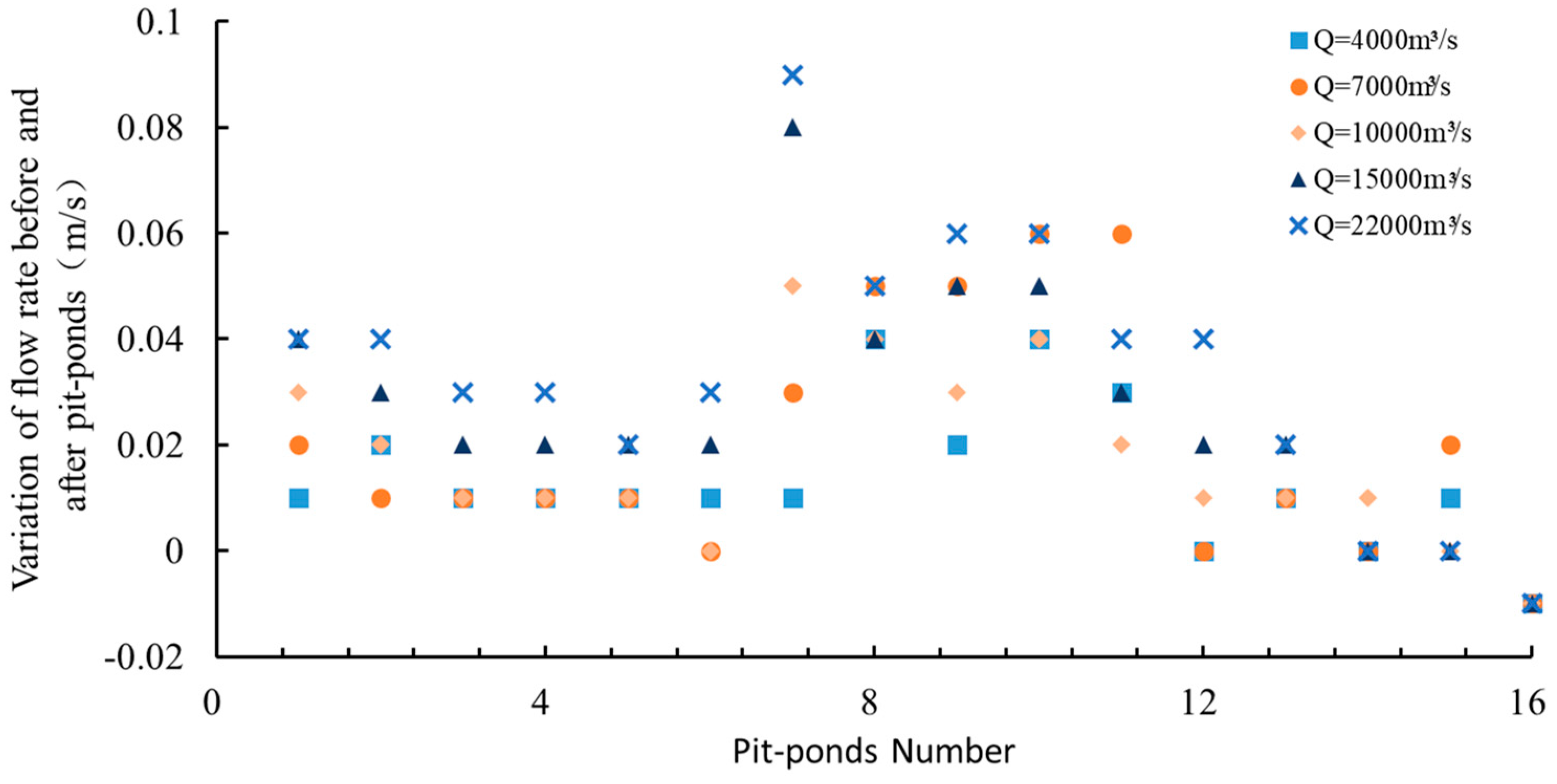
(2) Changes in flow velocity
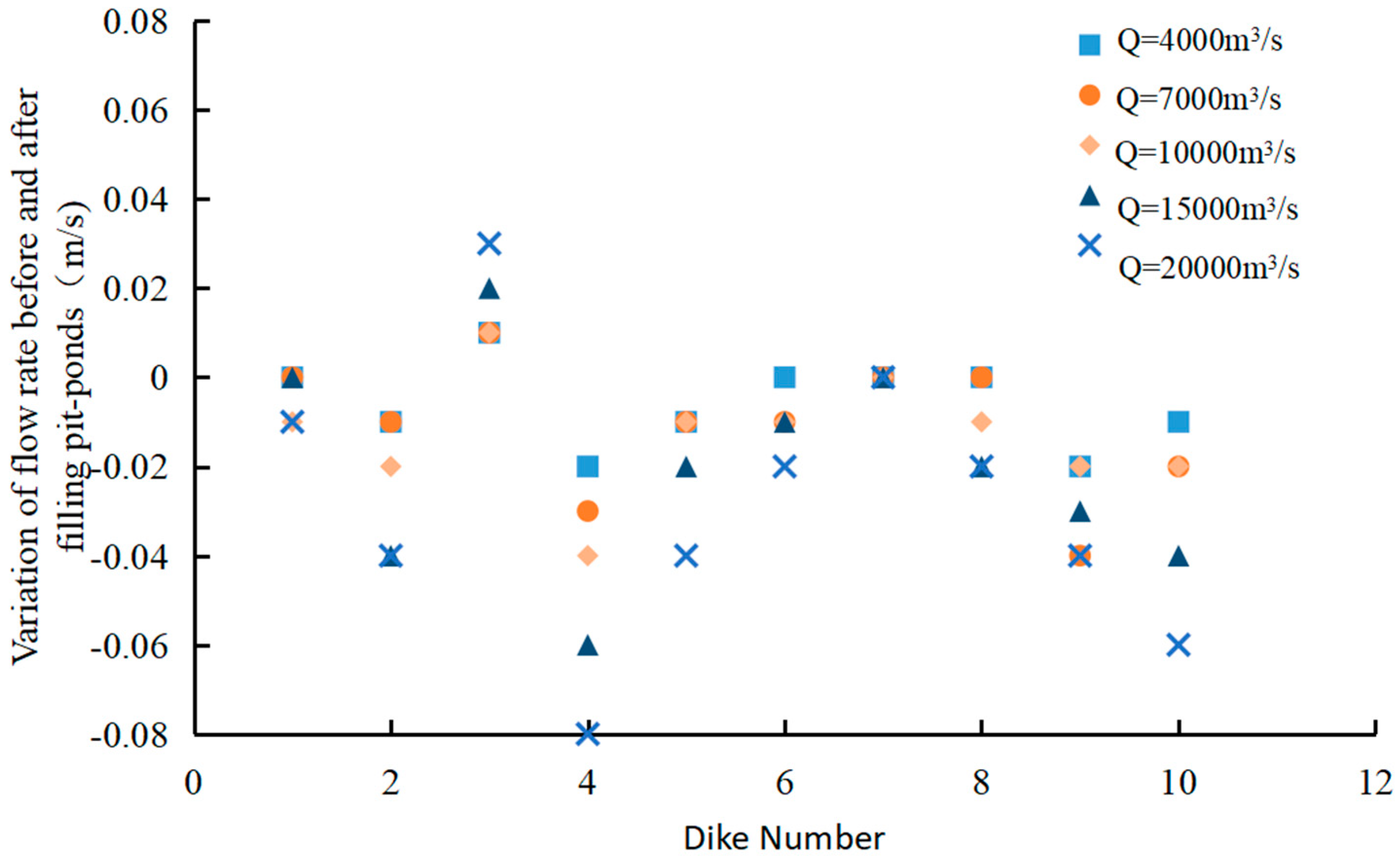
Under various computational operating conditions, changes in the velocity of the pit-pond points are shown in Figure 7, and changes in the velocity around the spur dike are shown in Figure 8. It can be seen that the flow velocity of local waters has been adjusted after backfilling. The depth of water at each measuring point in the pit-ponds has decreased, and the flow velocity has slightly increased, but the overall change is small. The flow velocity of the measuring point in the front waters around the spur dike decreased slightly, but the change is relatively smaller. Under the condition of Q = 2200 m3/s, the increase in the flow velocity in the pit-ponds is small after the implementation of backfilling, generally within 0.1 m/s. The flow velocity at the front of the spur dike in the flood protection project of the training dike flooding has been slightly reduced, with the amplitude generally within 0.08 m/s.
(3) Change in flow velocity distribution
The distribution of cross-sectional velocity before and after filling the pit-ponds under Q = 7000 m3/s and 22,000 m3/s flow is shown in Figure 9 and Figure 10. It can be seen from the figure that the axis of hydrodynamic force has not changed basically after the implementation of the project. Only the local range velocity of the pit-pond backfilling area has been slightly adjusted, and the change of flow velocity in other areas is small.
Under the condition of Q = 7000 m3/s flow, the natural floodplain is stagnant for a long time, both sides of the main channel are basically submerged, but the beach flow rate is relatively small, generally within 0.4 m/s, and the flow rate in the pit-ponds after backfilling is generally within 0.07 m/s, and the change of flow velocity in other areas is small. Under the conditions of Q = 10,000 m3/s, Q = 15,000 m3/s, and Q = 2200 m3/s, it is a full-section flood. In general, the greater the flow volume, the greater the flow velocity, and the greater the impact of pit-pond backfilling. Under the condition of Q = 2200 m3/s, the maximum velocity of the beach is generally within 1.1 m/s, and the increase in the flow velocity in the pit-ponds after the implementation of backfilling is relatively small, generally within 0.1 m/s.
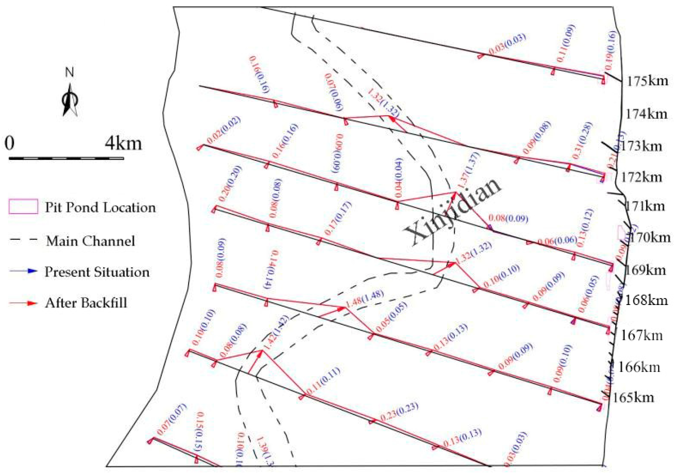
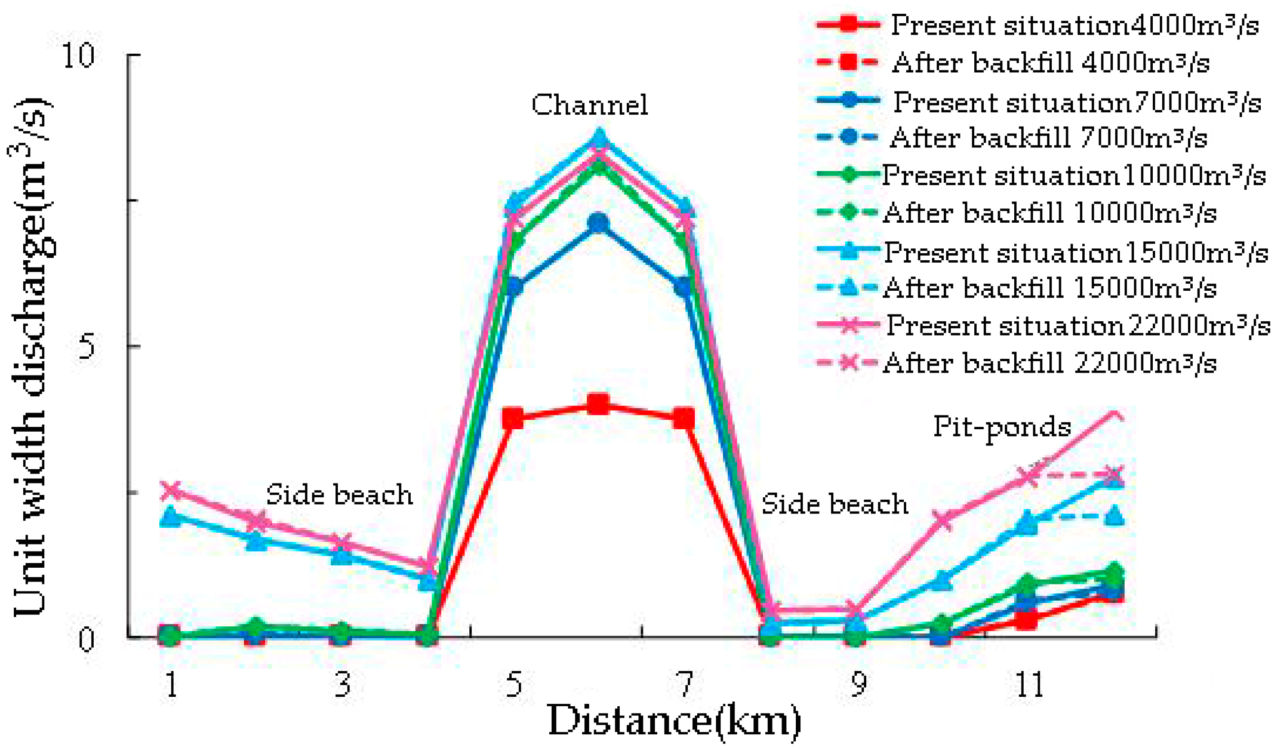
4.1.3. Influence of Backfilling in Pit-Ponds on Section Flow
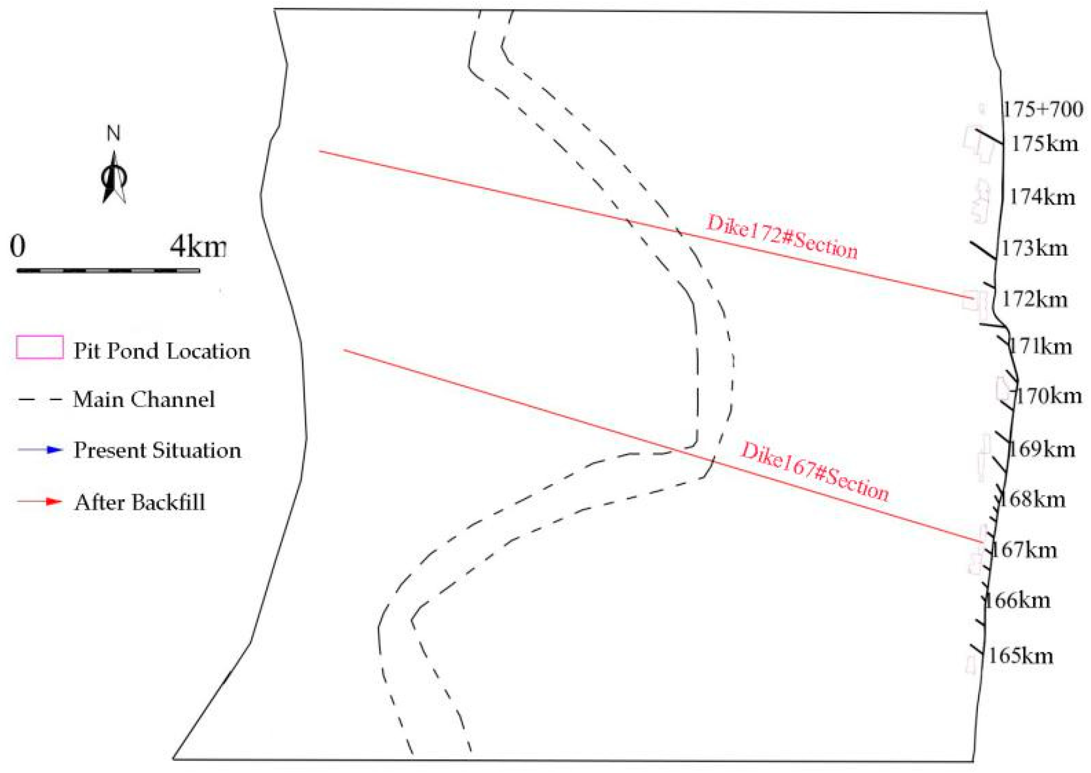
The two flow sections of the pit-ponds area are selected to analyze the impact of backfilling. The location of the cross-section is shown in Figure 11. The single width flow distribution of the cross-section is shown in Figure 12 and Figure 13. It can be seen from the figure that the main channel under each flow is the main channel for floods. Due to the obvious horizontal ratio drop on the banks on both sides of the main channel, the single width flow is generally closer to the root of the dike under various operating conditions, while the single width flow on both sides of the dike is larger than on other parts of the beach land. After filling the pond, there is no significant change in the single width flow in the section, the main channel, and the beach areas on both sides. The local single width flow in the backfilling area decreased, and the amplitude is generally within 30%.
4.2. Seepage, Anti-Sliding, and Seismic Resistance Safety Review
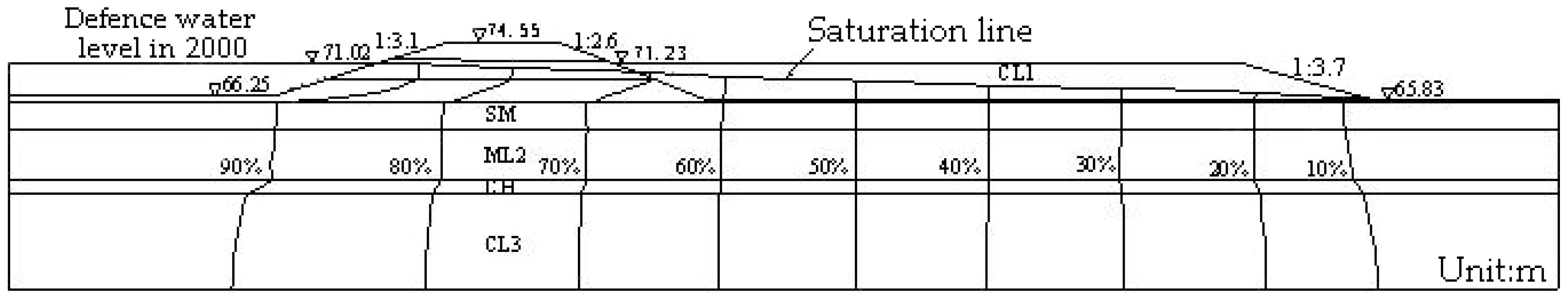
According to the Geological Survey data, six sections are selected as the calculation sections. Considering the length of this paper, only one of the sections is selected as an example. The simplified profile of the section is as Figure 14.
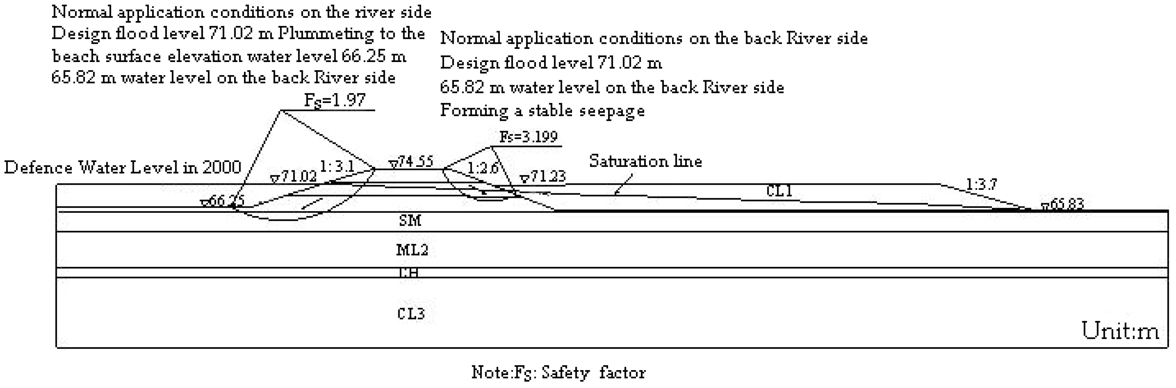
4.2.1. Seepage Safety Review
The operating condition of seepage calculation is shown in Figure 15. The water level of flood prevention is selected as water level on the riverside, while the ground elevation at the lowest point is selected as the water level on the back side. The results show that the seepage field of the dike is normal, the line of seepage does not escape from the slope surface of the silt area, and there is no seepage stability and safety problem on the slope surface. The total differential head between the front of the dike and the back slope of the dike is about 5.2–8.14 m. The seepage diameter at the contact surface of the dike is generally about 160 m, and the average falling gradient is about 0.051. The seepage stability of the dike satisfies the requirements. Due to the distance between the pit-ponds and the dike foot, there is no obvious effect on the seepage of the dike.
4.2.2. Anti-Sliding Safety Review
The selection of the section of the anti-sliding stability analysis, the calculation conditions, and the seepage analysis are the same. The simplified Bishop method is used as the calculation method, and the arc sliding surface is selected for analysis. The calculation results of the typical section are shown in Figure 16. The anti-sliding stability safety factor of the dike slope on the riverside and back side of the river under the section is greater than the minimum value of 1.2 specified in the specification. Because the pit pond has a certain distance from the foot of the dike, the stability of the slope is not affected. The calculation of the anti-sliding safety review also shows that the slope under various working conditions is stable and there will be no landslide danger.
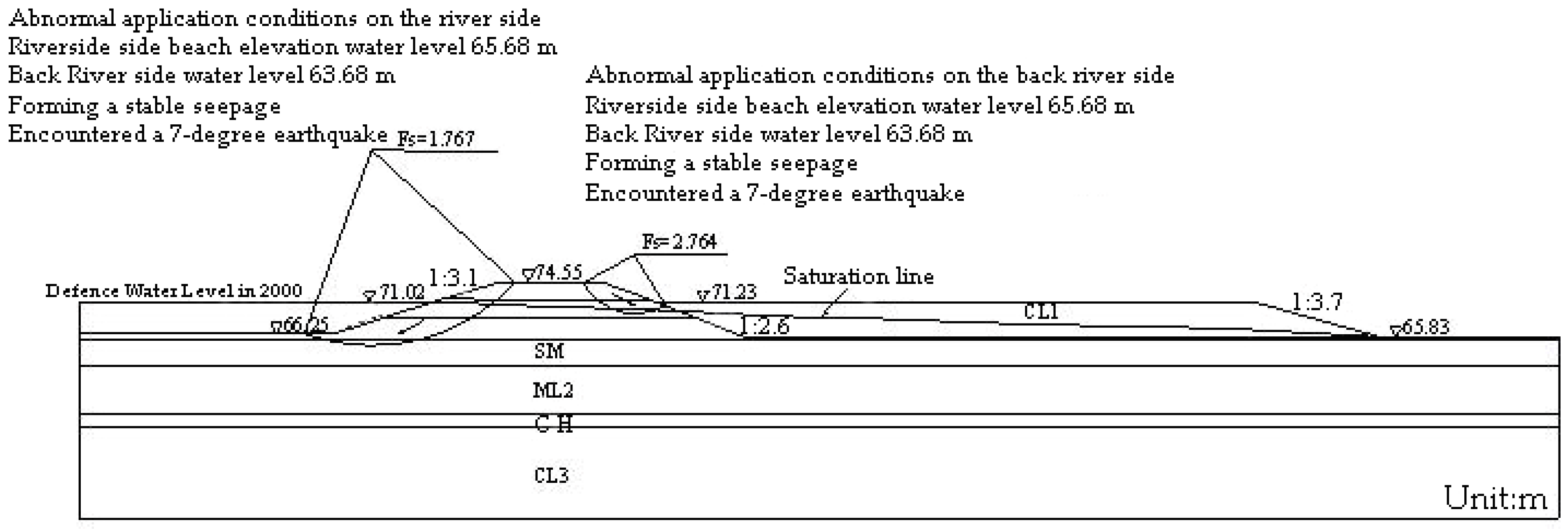
4.2.3. Seismic Resistance Safety Review
Seismic resistance stability analysis section selection and seepage analysis are the same, the calculation conditions are non-conventional operating conditions (the multi-year average water level on the riverside, and 7-degree earthquake is encountered by taking the ground elevation on the back side of the river to form a stable seepage), and the calculation method is the same as the anti-sliding safety review. The results of the calculation of the typical section are shown in Figure 17. The seismic resistance stability safety of the dike on the riverside and backside of the river is greater than the minimum value of 1.5 specified in the specification. There are pit ponds on the back river side of the dike, because of the existence of the pit pond, which changes the original terrain and increases the height difference of the ground on the back river of the levee, which may affect the seismic safety of the dike project. The seismic safety review calculation also shows that the section dike on the side of the river must equal the back of the dike seismic stability and safety to meet the review of seismic safety.
4.3. Project Flood Control Safety Evaluation
Through hydrodynamic analysis and seepage, anti-sliding, and seismic resistance safety review, the following conclusions can be drawn. The pit-ponds on the riverside have no obvious effect on the water flow in the dike area; simultaneously, due to the distance between the pit-ponds and the dike, the seepage, anti-sliding, and seismic resistance safety of the dike have not been significantly affected, which satisfies the requirements of the standard. Therefore, the flood control safety of the dike meets the requirements.
5. Conclusions
Based on momentum equation and continuous equation, the two-dimensional flow mathematical model is established, and the accuracy of the model in the analysis of river hydrodynamics is verified by an example. The model is applied to the analysis of flood impact of potholes on a river channel, and combined with seepage, anti-sliding, and seismic resistance safety review of dikes, the impact of riverside pit-ponds on flood control safety is evaluated. Taking a section of the Yellow River riverside pit-ponds as an example, the water level, flow velocity, and flow volume of the river after the floodplain under the current conditions and the backfilling conditions of the pit-ponds are simulated. The results show that the existence of the pit-ponds only affects the hydrological factors in the vicinity of the pit-ponds and the impact is small, and will not threaten the flood control safety of the area. Through the flood control safety evaluation of the project, it is shown that the two-dimensional water flow mathematical model combined with seepage, anti-sliding, and seismic resistance safety review can be used to comprehensively evaluate the flood control safety of dikes.
The water conservancy project has the functions of agricultural irrigation, flood control and drought resistance, and river operation, and is the basic guarantee for the sustained growth of the social economy. As an indispensable part of water conservancy projects, dikes should correctly treat dike flood control safety. Due to the existence of pit-ponds, the original terrain has been changed, which may have a certain impact on the flood control safety of the dike project. The method of this paper expands the related numerical research of dike pits and provides a new idea for flood control safety evaluation of similar projects. In the subsequent research, other numerical simulation methods can be tried to improve the calculation speed to obtain more accurate results, and can be applied to flood control safety evaluation in various fields, such as hydraulic engineering.
Author Contributions
Conceptualization, S.L. and D.Y.; methodology and software, S.L. and D.Y.; writing—original draft preparation, S.L.; formal analysis, D.Y.; writing—review and editing, J.S., C.X., and Y.C.; supervision, J.S. and J.C. All authors have made contributions to this work.
Funding
This research was funded by the National Key Research and Development Program of China (Grant No. 2017YFC0404806).
Conflicts of Interest
The authors declare no conflict of interest.
References
- Ministry of Water Resources of the People’s Republic of China. The First National Water Resources Census Bulletin; China Water & Power Press: Beijing, China, 2012.
- Gu, H. Water Conservancy Brilliant 50 Years; China Water & Power Press: Beijing, China, 1999; Volume 12, pp. 1–285. [Google Scholar]
- Miao, C.Y. Analysis of the influence of dike rivers and pit-ponds near the dike in the downstream of the Yellow River. Yellow River 2004, 1, 9–11. [Google Scholar]
- Loc, P. Environmental impact on the development of agricultural technology in China: The case of the dike-pond system of integrated agriculture-aquaculture in the Zhujiang Delta of China. Agric. Ecosyst. Environ. 1996, 60, 183–195. [Google Scholar]
- Zhao, S.G.; Cang, X.Q.; Geng, Y. The Assessment about the Impact of Landside Pit-Ponds of the Yellow River on Hydrological Safety of the Dike. Chinese Hydraulic Engineering Society, Advances in Research and Application of Hydraulic Seepage—Proceedings of the Fifth National Conference on Hydraulic Seepage; The Yellow River Water Conservancy Press: Zhenzhou, China, 2006; pp. 323–327. [Google Scholar]
- Yang, C.G.; Su, W.T.; Chen, Y.P. The application analysis of the anti-seepage technology by filling pond on river regulation. Henan Water Conserv. South-To-North Water Transf. Proj. 2015, 4, 24–25. [Google Scholar]
- Song, L.X.; Yang, F.; Hu, X.Z. A coupled mathematical model for two-dimensional flow-transport simulation in tidal river network. Adv. Water Sci. 2014, 25, 550–559. [Google Scholar]
- Wang, C.H.; Xiang, X.H. Generic 2-D river network numerical model. Adv. Water Sci. 2007, 18, 516–522. [Google Scholar]
- Bai, Y.C.; Yang, J.M.; Huang, B.S. Application of 2-D mathematical model in training of complicated river channel. J. Hydraul. Eng. 2003, 34, 25–30. [Google Scholar]
- Zhou, W.; Gao, H.C.; Wu, T. Application of 2-D Numerical Model of Bed Load in Rivers of Mountain Area: Regulation Project in Wangmo River as An Example. J. Yangtze River Sci. Res. Inst. 2016, 33, 6–10. [Google Scholar]
- Dong, Y.H. Review and Prospect of CRSRI Mathematical Models of River Flow and Sediment Transport. J. Yangtze River Sci. Res. Inst. 2011, 28, 7–16. [Google Scholar]
- Shi, Y.B.; Pan, C.H.; Cheng, W.L. 2D movable-bed mathematical model for dam-break flow and sediment transport. J. Hydraul. Eng. 2012, 43, 834–841+851. [Google Scholar]
- Jiang, X.M.; Li, D.X.; Wang, X.K. Coupled one-and two-dimensional numerical modeling of levee-breach flows using the Godunov method. Adv. Water Sci. 2012, 23, 214–221. [Google Scholar]
- Tayefi, V.; Lane, S.N.; Hardy, R.J. A comparison of one-and two-dimensional approaches to modelling flood inundation over complex upland floodplains. Hydrol. Process. 2010, 21, 3190–3202. [Google Scholar] [CrossRef]
- Sun, D.P.; Liao, X.L.; Wang, P.T. Influence of productive dikes on river flooding by 2-D Numerical simulation. J. Hydrodynam. 2007, 22, 24–30. [Google Scholar]
- Bates, P.D.; Anderson, M.G.; Baird, L. Modelling floodplain flow with a two-dimensional finite element scheme. Earth Surf. Process. Landf. 1992, 17, 575–588. [Google Scholar] [CrossRef]
- Xu, H.; Li, G.B.; Shang, Q.Q. A new numerical simulation approach for 2-D flow with submerged spur-dikes. Adv. Water Sci. 2014, 25, 407–413. [Google Scholar]
- Xie, L. Study on Compound Hydrodynamic Conditions in Terminal of Fluctuating Backwater Reach of Three Gorge Reservoir and Its Influence of Sediment Transport; Chongqing Jiaotong University: Chongqing, China, 2013. [Google Scholar]
- Wu, D.W.; Wang, X.D.; Wang, X.J. Research on regulation parameters of waterway in sansha river section of Yangtze river. In Chinese Society for Oceanography, Proceedings of the 16th China Ocean (Coastal) Engineering Symposium; China Ocean Press: Beijing, China, 2013; pp. 519–524. [Google Scholar]
Figure 1.
Grid diagram of the river section.

Figure 2.
Discrete topographic map of the river section.

Figure 3.
Comparison of measured and calculated water levels.

Figure 4.
Comparison of flood water level in the present condition and the backfilling condition.

Figure 5.
Variation of flow field under the floodplain condition (Q = 7000 m3/s).

Figure 6.
Variation of flow field under the floodplain condition (Q = 22,000 m3/s).

Figure 7.
The variation of velocity in the pit-ponds.

Figure 8.
Variation of the velocity around the spur dike.

Figure 9.
The velocity distribution under the floodplain condition (Q = 7000 m3/s).

Figure 10.
The velocity distribution under the floodplain condition (Q = 22,000 m3/s).

Figure 11.
The cross-section position.

Figure 12.
Single width flow distribution of the 167 cross-section.

Figure 13.
Single width flow distribution of the 172 cross-section.

Figure 14.
Typical profile map of the dike.

Figure 15.
Seepage field potential distribution diagram of typical dike section.

Figure 16.
Calculation result of anti-sliding stability of typical dike section.

Figure 17.
Calculation results of seismic stability of typical dike section.

© 2019 by the authors. Licensee MDPI, Basel, Switzerland. This article is an open access article distributed under the terms and conditions of the Creative Commons Attribution (CC BY) license (http://creativecommons.org/licenses/by/4.0/).
Share and Cite
MDPI and ACS Style
Liu, S.; Yang, D.; Sheng, J.; Chen, J.; Xu, C.; Chen, Y. Study on the Assessment Method of the Impact on Hydrological Safety of Riverside Pit-Ponds along a Dike. Water 2019, 11, 744. https://doi.org/10.3390/w11040744
AMA Style
Liu S, Yang D, Sheng J, Chen J, Xu C, Chen Y. Study on the Assessment Method of the Impact on Hydrological Safety of Riverside Pit-Ponds along a Dike. Water. 2019; 11(4):744. https://doi.org/10.3390/w11040744
Chicago/Turabian StyleLiu, Shuai, Dewei Yang, Jinbao Sheng, Jiankang Chen, Chengjun Xu, and Yingying Chen. 2019. "Study on the Assessment Method of the Impact on Hydrological Safety of Riverside Pit-Ponds along a Dike" Water 11, no. 4: 744. https://doi.org/10.3390/w11040744
Note that from the first issue of 2016, this journal uses article numbers instead of page numbers. See further details here.