Watershed Characterization and Hydrograph Recession Analysis: A Comparative Look at a Karst vs. Non-Karst Watershed and Implications for Groundwater Resources in Gaolan River Basin, Southern China


Abstract
:1. Introduction
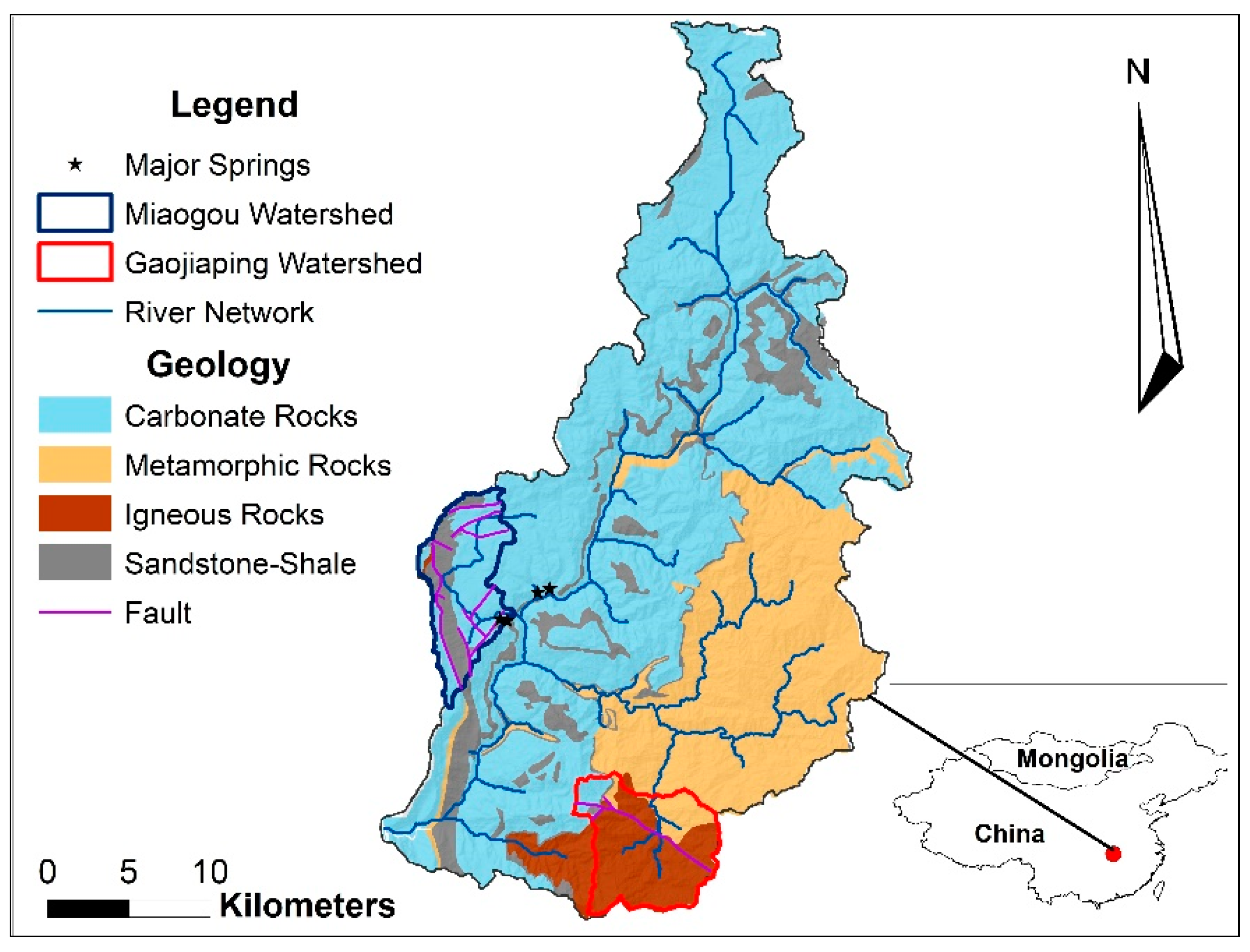
Study Area
2. Data and Methods
2.1. GIS Watershed Characterization
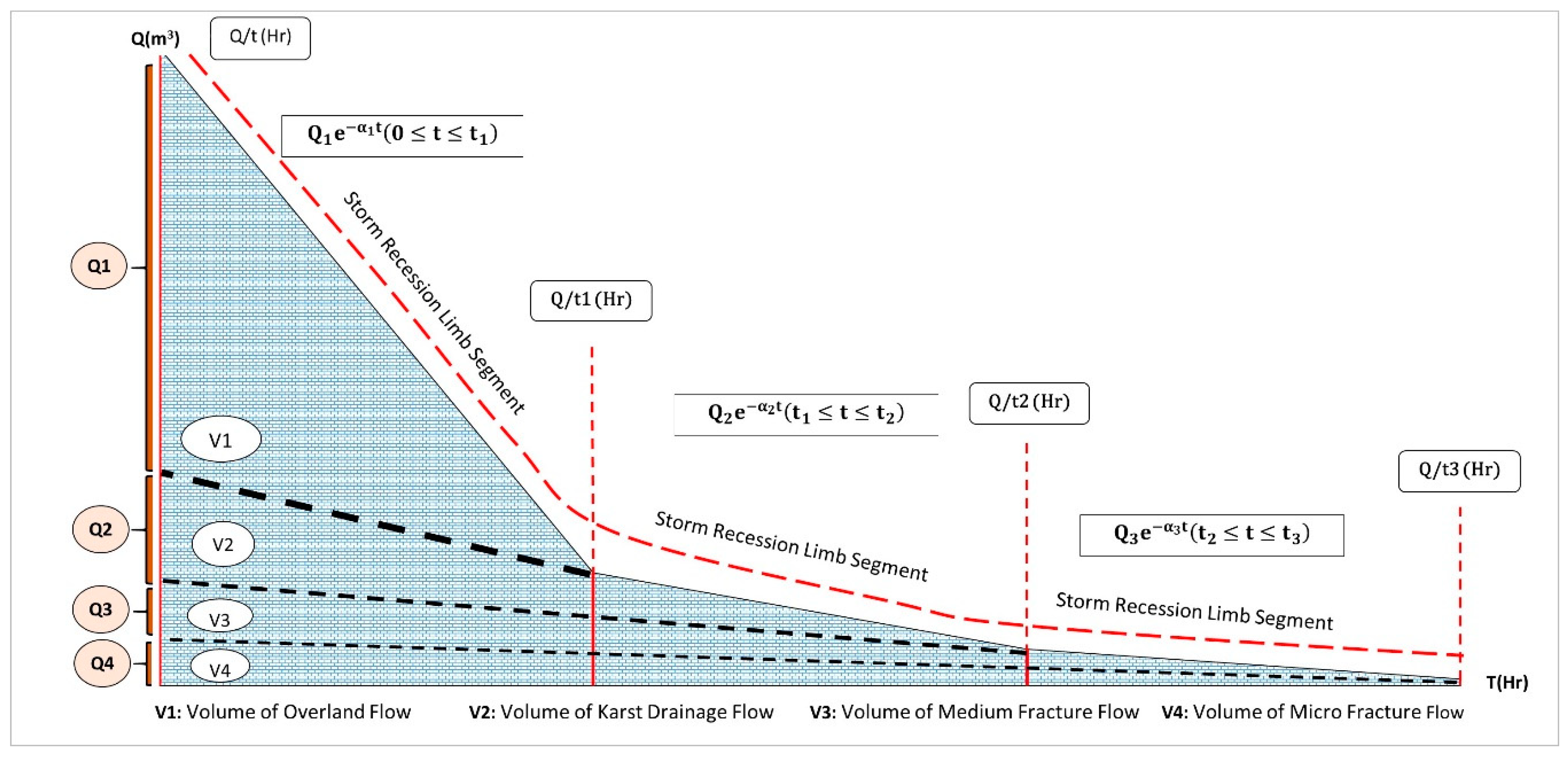
2.2. Hydrograph Recession Curve Analysis
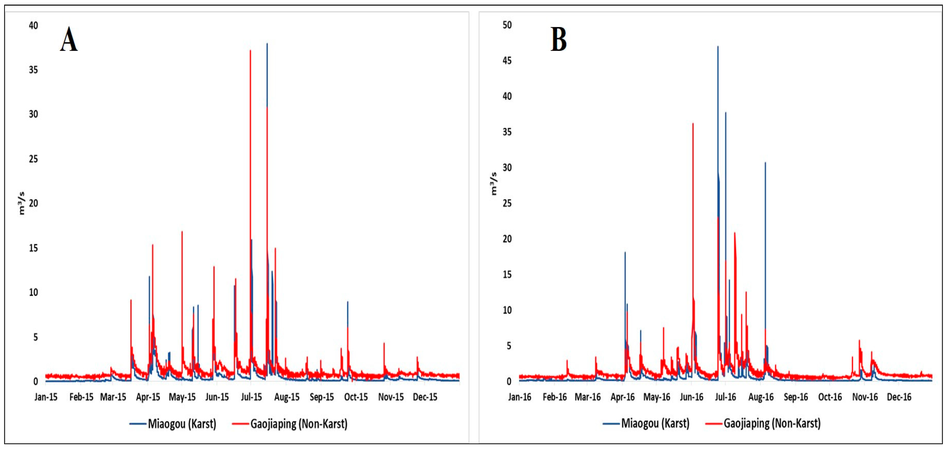
2.3. Streamflow Data
3. Results and Discussion
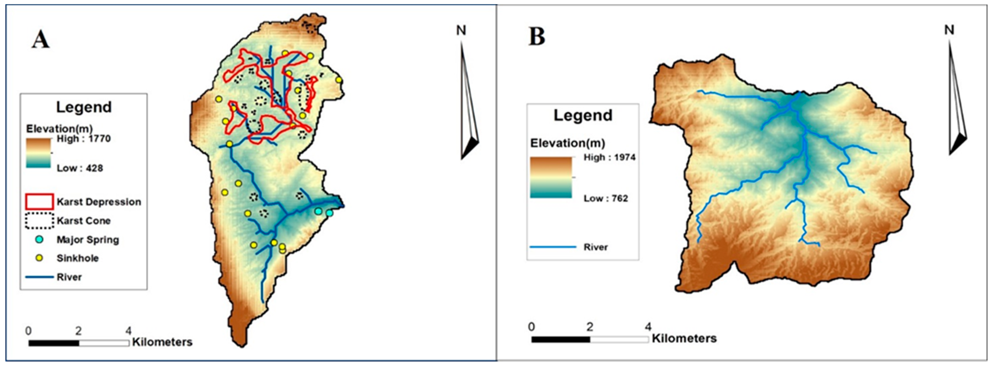
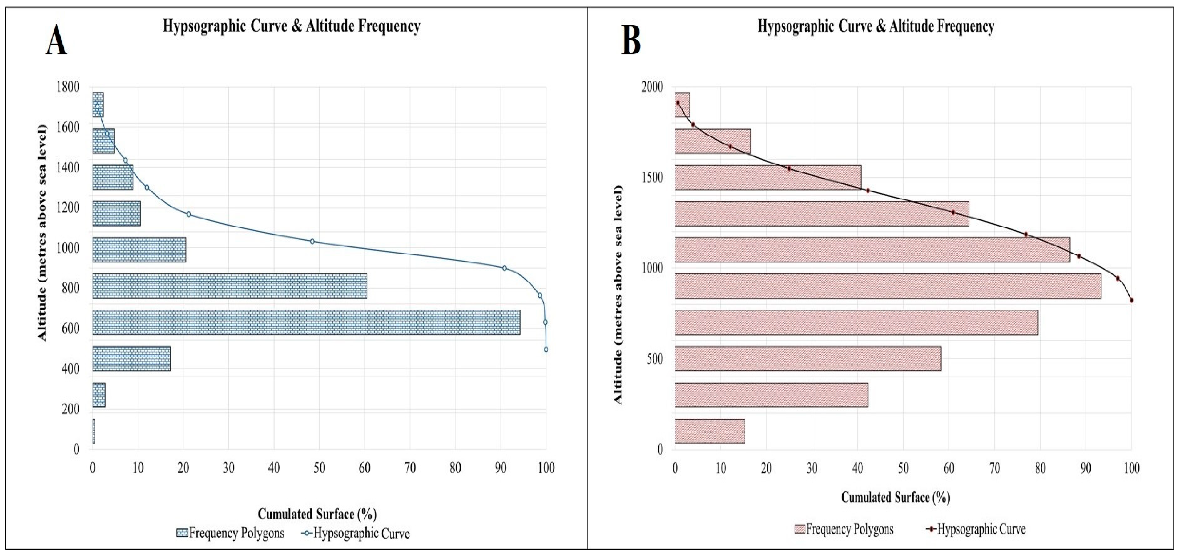
3.1. Topographic Analysis
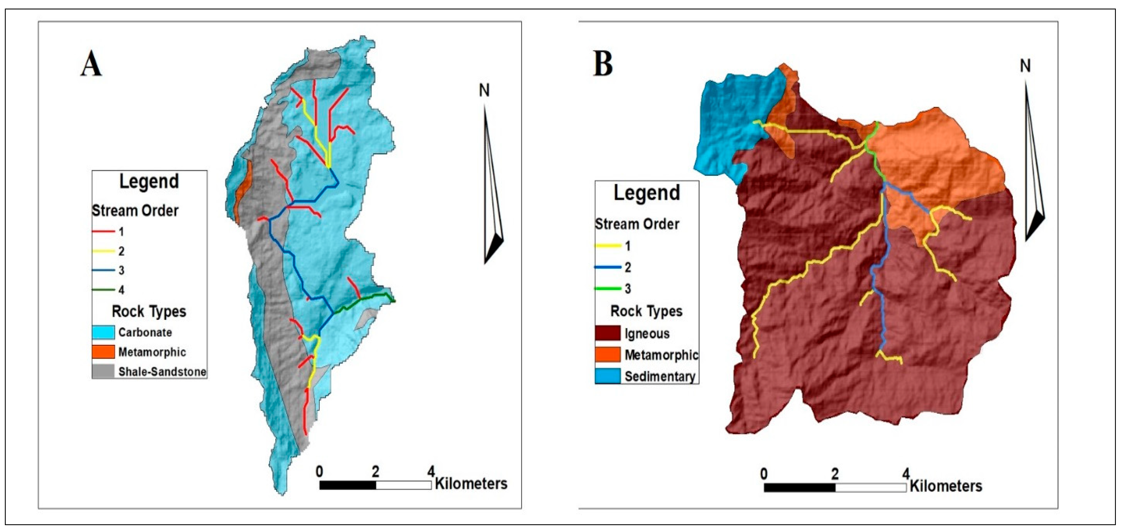
3.2. Drainage Network Analysis
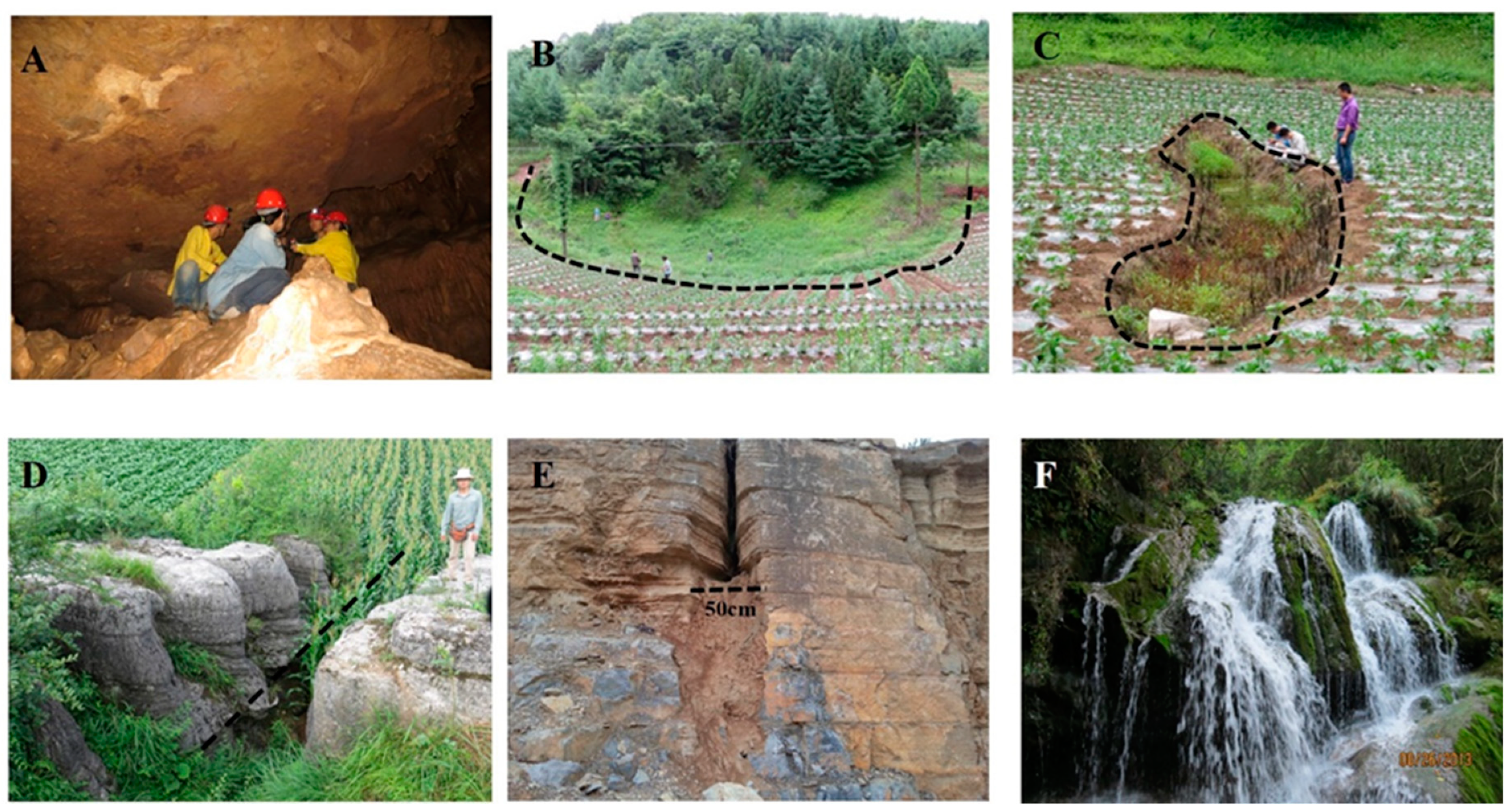
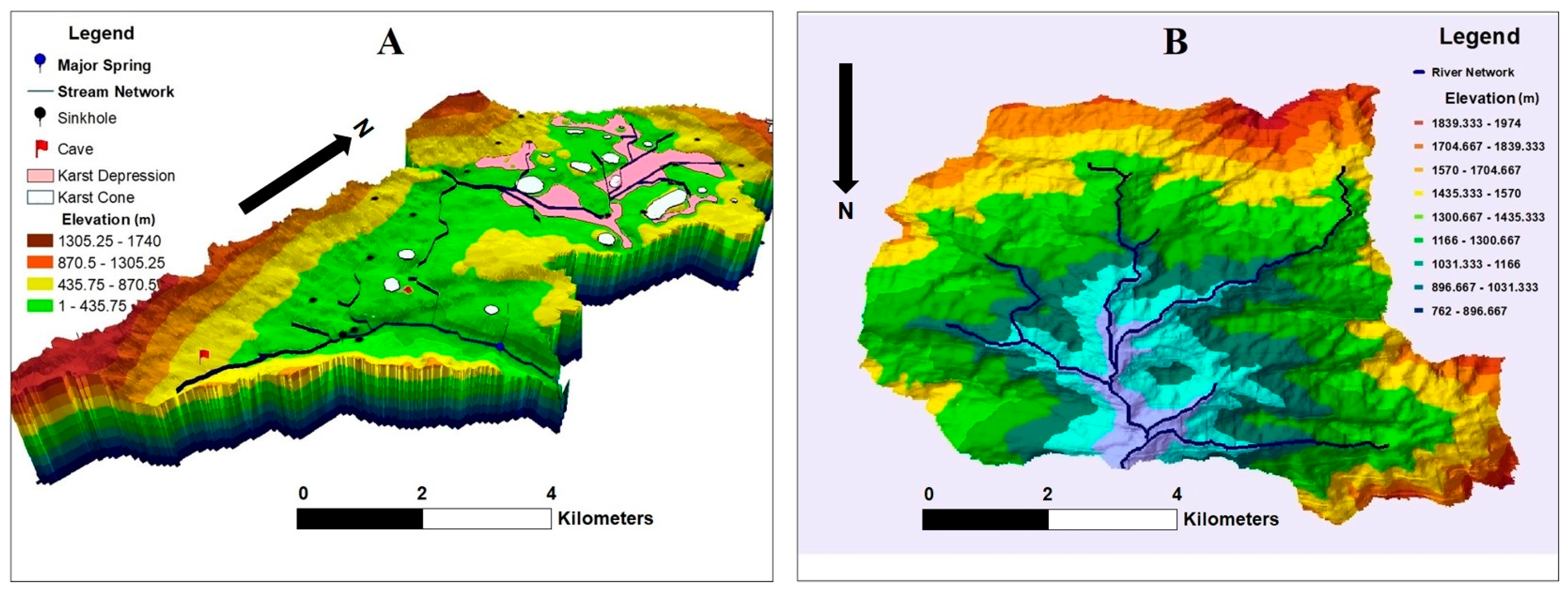
3.3. Geomorphic Analysis
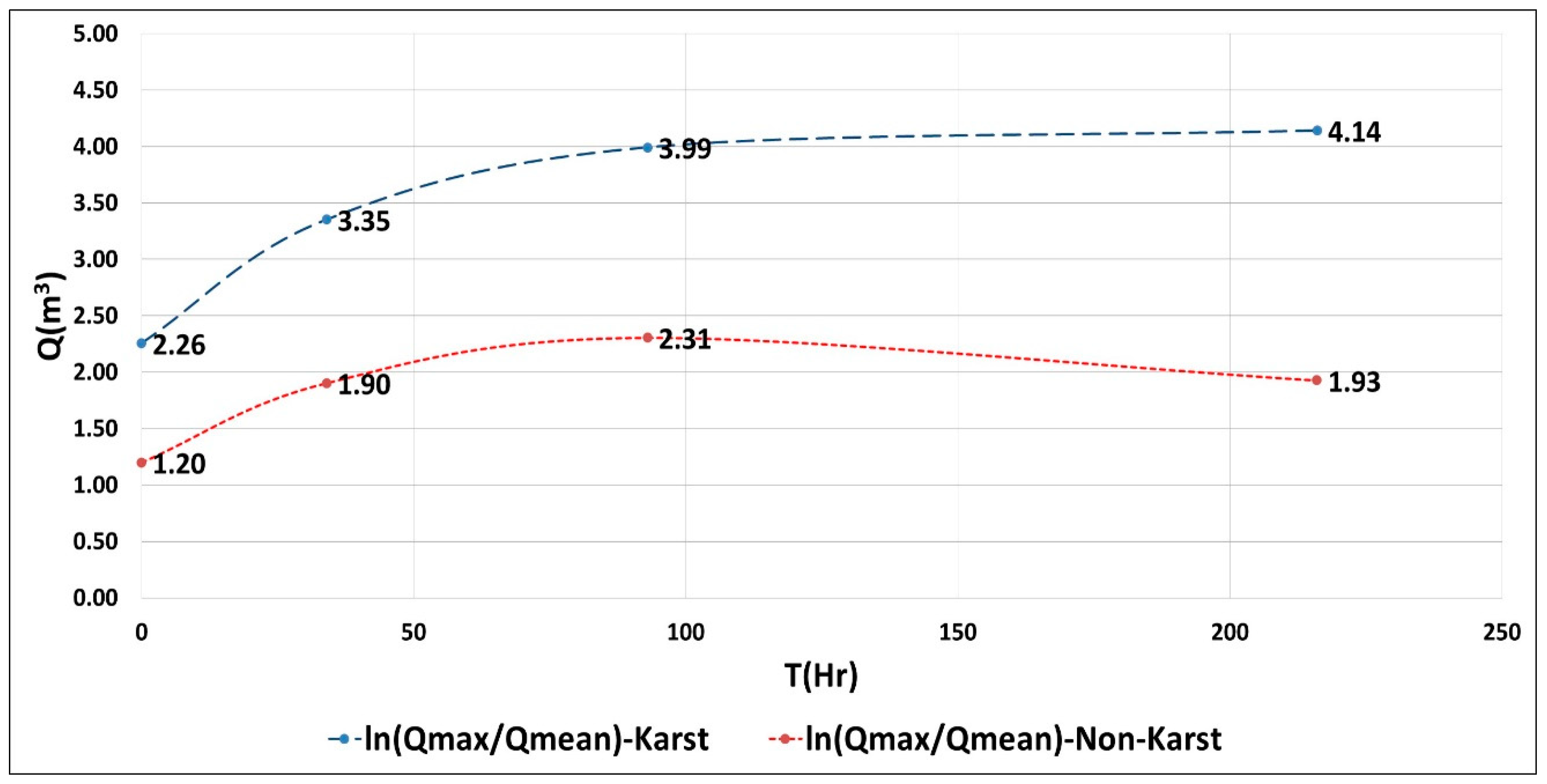
3.4. Hydrograph Recession Coefficient (α) Estimation
3.5. ANOVA on Recession Coefficient
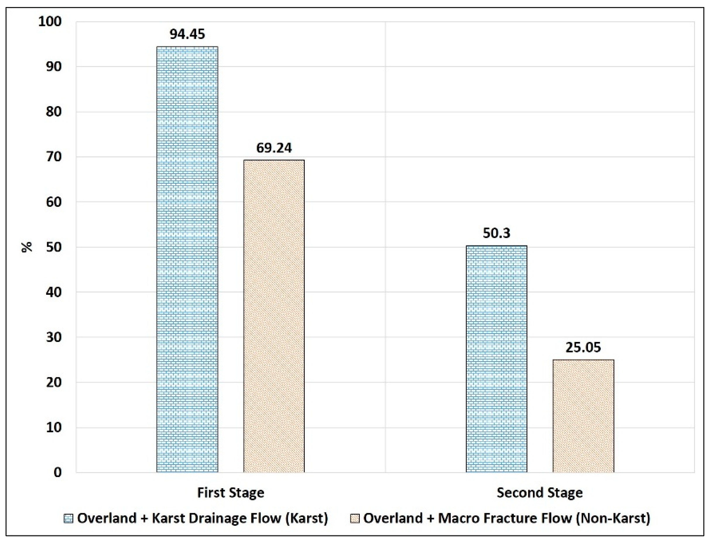
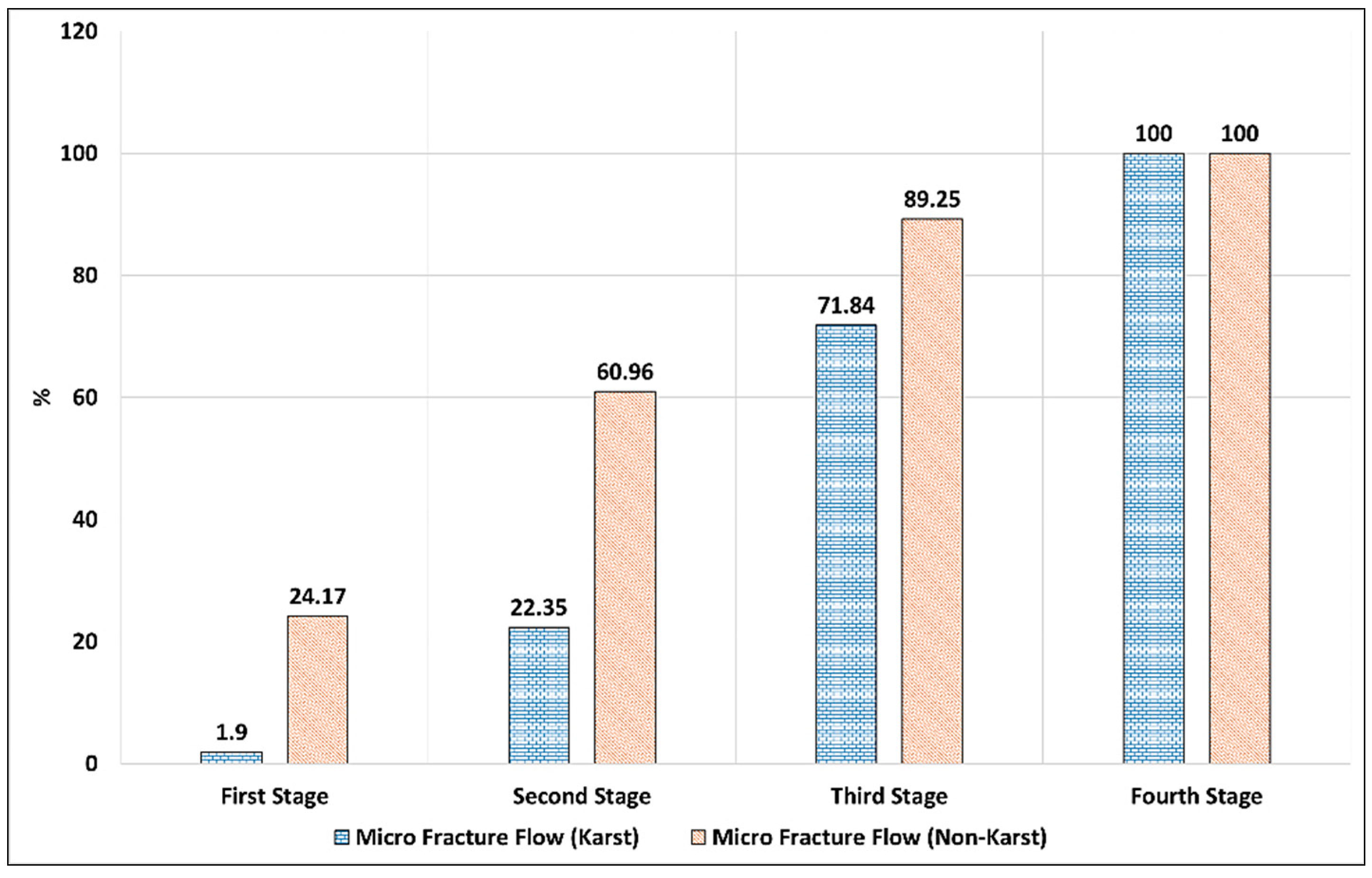
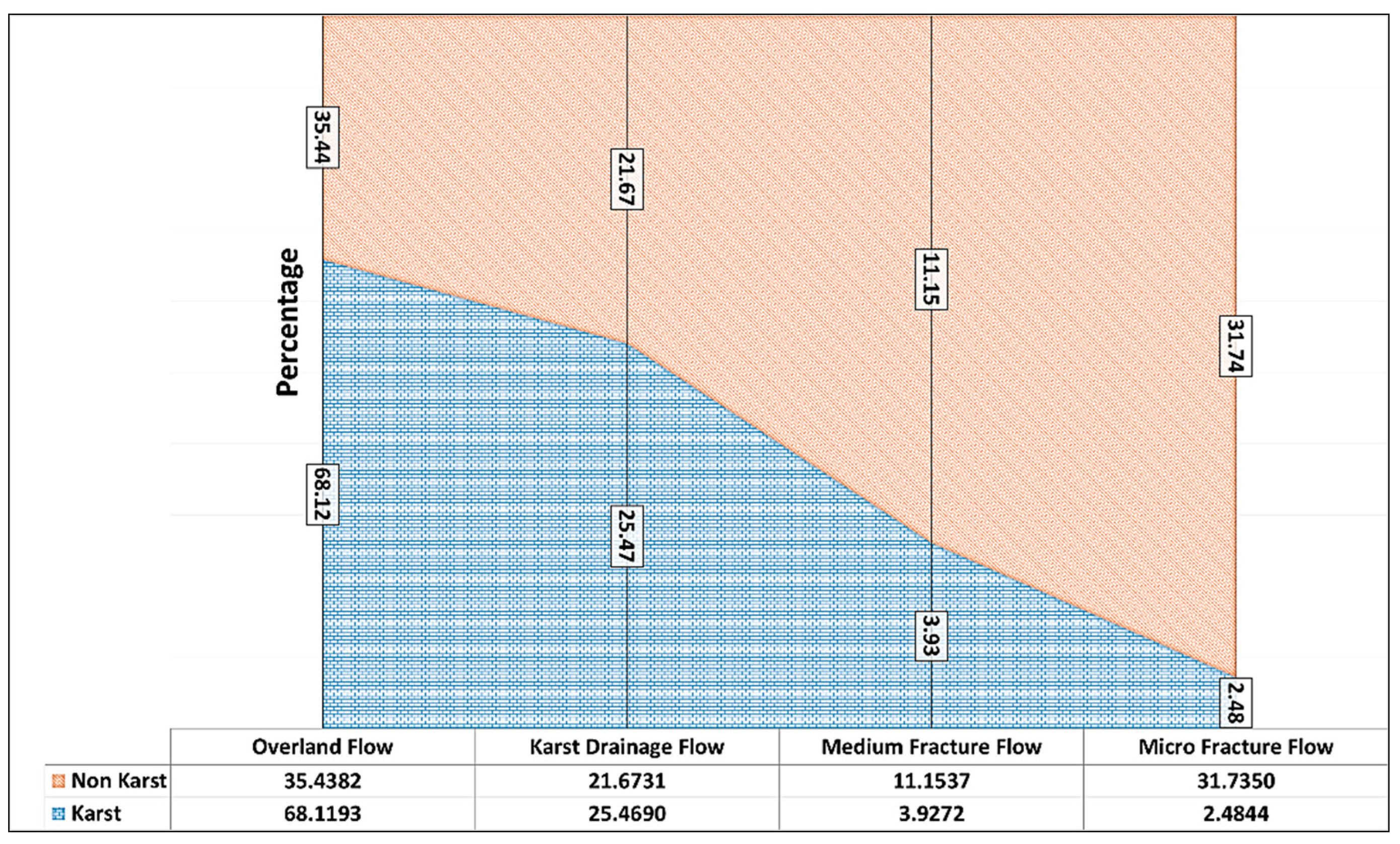
3.6. Streamflow Component Separation
3.7. Implications on Groundwater Availability and Quality in Karst Areas
4. Conclusions
Author Contributions
Funding
Conflicts of Interest
References
- Hartmann, A.; Goldscheider, N.; Wagener, T.; Lange, J.; Weiler, M. Karst water resources in a changing world: Review of hydrological modeling approaches. Rev. Geophys. 2014, 52, 218–242. [Google Scholar] [CrossRef]
- Ford, D.; Williams, P. Karst Hydrogeology and Geomorphology; John Wiley and Sons: Hoboken, NJ, USA, 2007; ISBN 978-0-470-84996-5. [Google Scholar]
- Stephen, R.; Jeannin, P.Y.; Alexander, E.C.; Davies, G.J.; Schindel, G.M. Contrasting definitions for the term ‘karst aquifer’. Hydrogeol. J. 2017, 25, 1237–1240. [Google Scholar] [CrossRef]
- Kresic, N.; Mikszweski, A. Hydrogeological Conceptual Site Models: Data Analysis and Visualization; CRC Press: Boca Raton, FL, USA, 2013. [Google Scholar]
- Jakada, H.; Chen, Z.; Luo, Z.; Zhou, H.; Luo, M.; Ibrahim, A.; Tanko, N. Coupling Intrinsic Vulnerability Mapping and Tracer Test for Source Vulnerability and Risk Assessment in a Karst Catchment Based on EPIK Method: A Case Study for the Xingshan County, Southern China. Arab. J. Sci. Eng. 2018, 44, 377–389. [Google Scholar] [CrossRef]
- Singhal, B.B.S. Nature of Hard Rock Aquifers: Hydrogeological Uncertainties and Ambiguities. In Groundwater Dynamics in Hardrock Aquifers; Ahmed, S., Jayakumar, R., Salih, A., Eds.; Springer: Dordrecht, Germany, 2008. [Google Scholar] [CrossRef]
- Price, K. Effects of watershed topography, soils, land use, and climate on baseflow hydrology in humid regions: A review. Prog. Phys. Geogr. Earth Environ. 2011, 35, 465–492. [Google Scholar] [CrossRef]
- Christina, T.; Gordon, G.E. A geological framework for interpreting the low-flow regimes of Cascade streams. Willamette River Basin Oregon Water Resour. Res. 2004, 40, W04303. [Google Scholar]
- Clark, M.P.; Rupp, D.E.; Woods, R.A.; Meerveld, H.J.T.-V.; Peters, N.E.; Freer, J.E. Consistency between hydrological models and field observations: Linking processes at the hillslope scale to hydrological responses at the watershed scale. Hydrol. Process. 2009, 23, 311–319. [Google Scholar] [CrossRef]
- Sayama, T.; McDonnell, J.J.; Dhakal, A.; Sullivan, K. How much water can a watershed store? Hydrol. Process. 2011, 25, 3899–3908. [Google Scholar] [CrossRef]
- Avdagić, I. Oticanje u Kraškim Hidrološkim Sistemima (Modelling of Runoff from Karstic Catchments). Ph.D. Thesis, Sarajevo University, Sarajevo, Yugoslavia, 1987. [Google Scholar]
- Bonacci, O. Karst Hydrology; Springer: Herdelberg, Germany, 1987. [Google Scholar]
- Bonacci, O.; Jelin, J. Identification of a karst hyrological system in the Dinaric karst (Yugoslavia). Hydrol. Sci. J. 1988, 33, 483–497. [Google Scholar] [CrossRef]
- Soulios, G. Contribution à l’étude des courbes de récession des sources karstiques: Exemples du pays Hellénique. J. Hydrol. 1991, 127, 29–42. [Google Scholar] [CrossRef]
- Kullman, E. Krasovo–Puklinové vody. Karst-Fissure Waters; Geologický ústav Dionýza Štúra: Bratislava, Czechoslovakia, 1990. [Google Scholar]
- Luo, M.; Chen, Z.; Yin, D.; Jakada, H.; Huang, H.; Zhou, H.; Wang, T. Surface flood and underground flood in Xiangxi River Karst Basin: Characteristics, models, and comparisons. J. Earth Sci. 2016, 27, 15–21. [Google Scholar] [CrossRef]
- Fiorillo, F.; Revellino, P.; Ventafridda, G. Karst aquifer draining during dry periods. J. Cave Stud. 2012, 74, 148–156. [Google Scholar] [CrossRef]
- Malik, P. Assessment of regional karstification degree and groundwater sensitivity to pollution using hydrograph analysis in the Velka Fatra Mountains, Slovakia. Environ. Earth Sci. 2006, 51, 707–711. [Google Scholar] [CrossRef]
- Pankaj, A.; Kumar, P. GIS-based morphometric analysis of five major sub-watersheds of Song River, Dehradun District, Uttarakhand with special reference to landslide incidences. J. Soc. Remote. Sens. 2009, 37, 157–166. [Google Scholar] [CrossRef]
- Doctor, D.H.; Young, J.A. An Evaluation of Automated GIS Tools for Delineating Karst Sinkholes and Closed Depressions from 1-Meter LIDAR-derived Digital Elevation Data. In Proceedings of the 13th Multidisciplinary Conference on Sinkholes and the Engineering and Environmental Impacts of Karst, Carlsbad, NM, USA, 6–10 May 2013. [Google Scholar]
- Prafull, S.; Ankit, G.; Madhulika, S. Hydrological inferences from the watershed analysis of water resource management using remote sensing and GIS techniques. Egypt. J. Remote Sens. Space Sci. 2014, 17, 111–121. [Google Scholar]
- Olivera, F.; Maidment, D. GIS for hydrologic data development for the design of highway drainage facilities. Transp. Res. Rec. 1998, 1625, 131–138. [Google Scholar] [CrossRef]
- Olivera, F.; Maidment, D. GIS tools for HMS modeling support. In Hydrologic and Hydraulic Modeling Support with Geographic Information Systems; Maidment, D., Djokic, D., Eds.; ESRI Press: Redlands, CA, USA, 2000; pp. 85–112. [Google Scholar]
- HEC. Geospatial Hydrologic Modeling Extension HEC-GeoHMS: Version 1.0 User’s Manual; Hydrologic Engineering Center (HEC) Technical Report No CPD-77; U.S. Army Corps of Engineers: Champaign, IL, USA, 2000.
- Oliveira, E.D.; Crestani, A. Physiographic characterization of the watershed of stream Jandaia, Jandaia do Sul/PR. Acta Geogra´Fica 2011, 5, 169–183. [Google Scholar]
- EPA. Better Assessment Science Integrating Point and Nonpoint Sources (BASINS): Version 3.0 User’s Manual; Office of Water Technical Report No EPA-823-B-01-001; Environmental Protection Agency: Washington, DC, USA, 2001.
- Di Luzio, M.; Srinivasan, R.; Arnold, J.G.; Neitsch, S.L. Soil and water assessment tool. In ArcView GIS Interface Manual: Version 2002; International Center for Tropical Agriculture: Cali, Colombia, 2002. [Google Scholar]
- Luzio, M.; Srinivasan, R.; Arnold, J.G. Integration of Watershed Tools and Swat Model into Basins. JAWRA J. Am. Resour. Assoc. 2002, 38, 1127–1141. [Google Scholar] [CrossRef]
- Dixon, B.; Uddameri, V. GIS and Geocomputation for Water Resource Science and Engineering; John Wiley & Sons, Ltd.: Hoboken, NJ, USA, 2016. [Google Scholar]
- Strahler, A.N. Quantitative Geomorphology of Drainage Basins and Channel Networks. In Hand Book of Applied Hydrology; Te Chow, V., Ed.; McGraw Hill Book Company: New York, NY, USA, 1964. [Google Scholar]
- O’Callaghan, J.F.; Mark, D.M. The extraction of drainage networks from digital elevation data. Comput. Vis. Graph. Process. 1984, 28, 323–344. [Google Scholar] [CrossRef]
- Jenson, S.K.; Domingue, J.O. Extracting topographic structure from digital elevation data for geographic information system analysis. Photogramm. Eng. Remote Sens. 1988, 54, 1593–1600. [Google Scholar]
- Jenson, S.K. Applications of hydrologic information automatically extracted from digital elevation models. Hydrol. Process. 1991, 5, 31–44. [Google Scholar] [CrossRef]
- Boussinesq, J. Recherches Théoriques sur l’écoulement des Nappes d’eau Infiltrées dans le sol et sur dÉbit de Sources. J. De Mathématiques Pures Et Appliquées 1904, 10, 5–78. [Google Scholar]
- Maillet, E. Essais d’Hydraulique Souterraine et Fluviale; Hermann: Paris, France, 1905. (In French) [Google Scholar]
- Kullman, E. Nové metodické prístupy k riešeniu ochrany a ochranných pásiem zdrojov podzemných vôd v horninových prostrediach s krasovo—puklinovou priepustnosťou [New methods in groundwater protection and delineation of protection zones in fissure-karst rock environment; in Slovak]. Podzemn. Voda 2000, 6, 31–41. [Google Scholar]
- Malík, P.; Vojtkova, S. Use of recession-curve analysis for estimation of karstification degree and its application in assessing overflow/underflow conditions in closely spaced karstic springs. Environ. Earth Sci. 2012, 65, 2245–2257. [Google Scholar] [CrossRef]
- Miao, Z.L.; Miao, Z.Z. Application of Recession Equation in Groundwater Studies. Investig. Sci. Technol. 1984, 5, 1–6. (In Chinese) [Google Scholar]
- Kresic, N.; Bonacci, O. Spring Discharge Hydrograph. In Groundwater Hydrology of Springs; Kresic, N., Stevanovic, Z., Eds.; Butterworth-Heinemann: Oxford, UK, 2010. [Google Scholar]
- Strahler, A.N. Dynamic basis of geomorphology. Geol. Soc. Am. Bull. 1952, 63, 923–938. [Google Scholar] [CrossRef]
- Lambert, A.R. Satellite Geology and Photogeomorphology: An Instructional Manual for Data Integration; Springer: Berlin/Heidelberg, Germany, 2011; pp. 78–79. ISBN 978-3-642-20607-8. [Google Scholar]
- Stevanovic, Z. Karst Aquifers—Characterization and Engineering. Prof. Pract. Earth Sci. 2015. [Google Scholar] [CrossRef]
- Fiorillo, F. Tank-reservoir drainage as a simulation of the recession limb of karst spring hydrographs. Hyogeol. J. 2011, 19, 1009–1019. [Google Scholar] [CrossRef]
- Bonacci, O. Karst springs hydrographs as indicators of karst aquifers. Hydrol. Sci. J. 1993, 38, 51–62. [Google Scholar] [CrossRef] [Green Version]
- Kovács, A.; Perrochet, P.; Király, L.; Jeannin, P. A quntitative method for characterization of karst aquifers based on the spring hydrograph analysis. J. Hydrol. 2005, 303, 152–164. [Google Scholar] [CrossRef]
- Florea, L.J.; Vacher, H. Springflow Hydrographs: Eogenetic vs. Telogenetic Karst. Ground Water 2006, 44, 352–361. [Google Scholar] [CrossRef]
- Fiorillo, F. The Recession of Spring Hydrographs, Focused on Karst Aquifers. Resour. Manag. 2014, 28, 1781–1805. [Google Scholar] [CrossRef]
- Birk, S.; Hergarten, S. Early recession behaviour of spring hydrographs. J. Hydrol. 2010, 387, 24–32. [Google Scholar] [CrossRef]
- Burger, A.; Pasquier, F. Prospection et captage d’eau par fprages dans la vallée de la Brevine (Jura Suisse). In Hydrogeology of Karstic Terrains; Burger, A., Dubertret, L., Eds.; UNESCO: Paris, France, 1984; Volume 1, pp. 145–149. [Google Scholar]
- Babushkina, V.D.; Lebedyanskaya, Z.P.; Plotnikov, I.I. The distinctive features of predicting total water discharge from deep-level mines in fissure and karst rocks. In Hydrogeology of Karstic Terrains; Burger, A., Dubertret, L., Eds.; UNESCO: Paris, France, 1984; Volume 1, pp. 229–232. [Google Scholar]
- Escolero, O.A.; Marin, L.E.; Steinich, B.; Pacheco, A.J.; Cabrera, S.A.; Alcocer, J. Development of a Protection Strategy of Karst Limestone Aquifers: The Merida Yucatan, Mexico Case Study. Resour. Manag. 2002, 16, 351–367. [Google Scholar]


| Domain | Parameter | Units | Karst | Non-Karst |
|---|---|---|---|---|
| Geomorphic | Dominant Geology | - | Sedimentary | Metamorphic |
| Sinkholes | - | 18 | 0 | |
| Caves | - | 4 | 0 | |
| Springs | - | 2 | 0 | |
| Basin Shape | - | High-Concavity | Low-Concavity | |
| Cone Cones | - | 19 | 0 | |
| Karst Depressions | - | 4 | 0 | |
| Topographic | Area (A) | km² | 45 | 54 |
| Perimeter (P) | km² | 46 | 43 | |
| Max. Altitude (ALTmax) | m | 1770 | 1968 | |
| Min. Altitude (ALTmin) | m | 430 | 762 | |
| Avg. Altitude (ALTavg) | m | 1099 | 1365 | |
| Total Relief (RTotal) | m | 1340 | 1206 | |
| Watershed average slope | % | 31 | 40.35 | |
| Most Frequent Altitude | m | 898 | 1304.70 | |
| Hydrographic | Gravelius’s Shape Index (Cg) | Un | 1.93 | 1.65 |
| Drainage Network Avg. Slope | % | 22.56 | 19.34 | |
| Main Channel Length (ML) | km | 15 | 11.91 | |
| Stream Order 1 Length | km | 14.23 | 16.80 | |
| Stream Order 2 Length | km | 5.63 | 6.35 | |
| Stream Order 3 Length | km | 8.47 | 1.91 | |
| Stream Order 4 Length | km | 2.53 | 0 | |
| Total Length of Drainage Network (Lt) | km | 30.86 | 25.06 | |
| Drainage Density (Dd) | km/km² | 0.68 | 0.46 | |
| Stream Density | 0.68 | 0.28 | ||
| Avg. Length of Surface Runoff | km | 0.36 | 0.54 |
| No | Peak Flow (m3/s) | Stage I | Stage II | Stage III | Stage IV | ||||||||
|---|---|---|---|---|---|---|---|---|---|---|---|---|---|
| α(1/h) | T(h) | Q1 | α(1/h) | T(h) | Q2 | α(1/h) | T(h) | Q3 | α(1/h) | T(h) | Q4 | ||
| 1 | 2.71 | 0.0760 | 26 | 0.38 | 0.0133 | 91 | 0.11 | 0.0036 | ≥216 | 0.05 | |||
| 2 | 9.71 | 0.0760 | 31 | 0.92 | 0.0113 | 95 | 0.31 | 0.0044 | 196 | 0.13 | 0.0006 | >132 | 0.12 |
| 3 | 19.86 | 0.1008 | 36 | 0.53 | 0.0149 | 86 | 0.51 | 0.0053 | >150 | 0.07 | |||
| 4 | 1.28 | 0.0972 | 19 | 0.20 | 0.0104 | 100 | 0.07 | 0.0043 | >162 | 0.04 | |||
| 5 | 12.65 | 0.0748 | 36 | 0.86 | 0.0154 | 94 | 0.20 | 0.0050 | >127 | 0.11 | |||
| 6 | 51.75 | 0.0535 | 53 | 3.04 | 0.0219 | 75 | 0.59 | 0.0041 | 195 | 0.26 | 0.0005 | >67 | 0.26 |
| 7 | 18.08 | 0.0775 | 36 | 1.11 | 0.0131 | 97 | 0.31 | 0.0038 | >122 | 0.20 | |||
| 8 | 3.35 | 0.0401 | 36 | 0.79 | 0.0085 | 88 | 0.37 | 0.0045 | >136 | 0.20 | |||
| 9 | 9.31 | 0.0751 | 26 | 1.32 | 0.0162 | 90 | 0.31 | 0.0020 | >70 | 0.27 | |||
| 10 | 14.93 | 0.0709 | 25 | 2.54 | 0.0094 | 109 | 0.91 | 0.0051 | >150 | 0.42 | |||
| 11 | 12.43 | 0.0537 | 47 | 1.00 | 0.0074 | 115 | 0.43 | 0.0026 | 260 | 0.22 | 0.0008 | >220 | 0.18 |
| 12 | 9.51 | 0.0839 | 35 | 0.50 | 0.0107 | 81 | 0.21 | 0.0021 | 279 | 0.12 | 0.0009 | >352 | 0.09 |
| 13 | 7.25 | 0.0481 | 47 | 0.76 | 0.0059 | 120 | 0.37 | 0.0032 | 197 | 0.20 | 0.0006 | >104 | 0.19 |
| 14 | 7.98 | 0.0539 | 28 | 1.76 | 0.0106 | 97 | 0.63 | 0.0047 | 172 | 0.28 | 0.0009 | >128 | 0.25 |
| 15 | 2.64 | 0.0434 | 30 | 0.72 | 0.0126 | 60 | 0.34 | 0.0033 | 212 | 0.17 | 0.0004 | ≥1858 | 0.08 |
| Average | 0.0683 | 34 | 0.79 | 0.0121 | 93 | 0.35 | 0.0039 | 216 | 0.18 | 0.0007 | 0.17 | ||
| Std Dev (σ) | 0.0187 | 9.3 | 0.79 | 0.004 | 15.1 | 0.22 | 0.0011 | 38.9 | 0.10 | 0.0002 | 0.07 | ||
| No | Peak Flow (m3/s) | Stage I | Stage II | Stage III | Stage IV | ||||||||
|---|---|---|---|---|---|---|---|---|---|---|---|---|---|
| α(1/h) | T(h) | Q1 | α(1/h) | T(h) | Q2 | α(1/h) | T(h) | Q3 | α(1/h) | T(h) | Q4 | ||
| 1 | 11.21 | 0.0444 | 27 | 3.38 | 0.0095 | 93 | 1.40 | 0.0065 | ≥128 | 0.61 | |||
| 2 | 41.39 | 0.0615 | 32 | 5.78 | 0.0150 | 70 | 2.02 | 0.0050 | >84 | 1.33 | |||
| 3 | 4.89 | 0.0195 | 27 | 2.89 | 0.0094 | 98 | 1.15 | 0.0024 | >87 | 0.93 | |||
| 4 | 2.37 | 0.0213 | 22 | 1.48 | 0.0044 | 119 | 0.88 | 0.0012 | 194 | 0.70 | 0.0002 | >185 | 0.67 |
| 5 | 7.27 | 0.0537 | 24 | 2.00 | 0.0075 | 74 | 1.15 | 0.0013 | 220 | 0.86 | 0.0006 | >294 | 0.72 |
| 6 | 1.79 | 0.0129 | 33 | 1.17 | 0.0030 | 109 | 0.84 | 0.0010 | 271 | 0.64 | 0.0002 | ≥1545 | 0.47 |
| 7 | 1.57 | 0.0072 | 47 | 1.12 | 0.0032 | 104 | 0.80 | 0.0014 | 210 | 0.60 | 0.0005 | >67 | 0.58 |
| 8 | 9.10 | 0.0630 | 22 | 2.28 | 0.0100 | 110 | 0.76 | 0.0025 | ≥219 | 0.44 | |||
| 9 | 15.33 | 0.0496 | 29 | 3.64 | 0.0108 | 108 | 1.13 | 0.0040 | ≥125 | 0.69 | |||
| 10 | 16.83 | 0.0373 | 33 | 4.91 | 0.0070 | 104 | 2.37 | 0.0036 | ≥97 | 1.67 | |||
| 11 | 7.51 | 0.0370 | 37 | 1.91 | 0.0037 | 96 | 1.34 | 0.0011 | ≥263 | 1.00 | |||
| 12 | 11.53 | 0.0536 | 28 | 2.57 | 0.0057 | 98 | 1.47 | 0.0019 | >120 | 1.17 | |||
| 13 | 37.18 | 0.0604 | 35 | 4.49 | 0.0059 | 89 | 2.66 | 0.0030 | ≥194 | 1.48 | |||
| 14 | 2.75 | 0.0270 | 35 | 1.07 | 0.0052 | 86 | 0.68 | 0.0007 | 285 | 0.56 | 0.0002 | ≥1729 | 0.40 |
| 15 | 36.16 | 0.0603 | 30 | 5.92 | 0.0143 | 75 | 2.03 | 0.0038 | 208 | 0.92 | 0.0005 | >96 | 0.88 |
| Average | 0.0405 | 31 | 2.97 | 0.0076 | 96 | 1.38 | 0.0026 | 235 | 0.91 | 0.0004 | 0.62 | ||
| Std Dev (σ) | 0.019 | 6.5 | 1.66 | 0.0038 | 14.5 | 0.62 | 0.0017 | 37.4 | 0.36 | 0.0002 | 0.17 | ||
| Miaogou | α, duration | 0.0535 | (0,54] | 0.0219 | (55,129] | 0.0041 | (130,324] | 0.0005 | (325,∞] | |
| Stages | Total | I | II | III | IV | |||||
| Flow Type | V,104 m3 | % | V,104 m3 | % | V,104 m3 | % | V,104 m3 | % | V,104 m3 | % |
| Overland Flow | 262.99 | 39.96 | 262.99 | 68.24 | ||||||
| Karst Drainage Flow | 124.06 | 18.85 | 101.94 | 26.45 | 22.12 | 50.30 | ||||
| Medium Fracture Flow | 34.54 | 5.25 | 13.15 | 3.41 | 12.02 | 27.35 | 9.37 | 28.16 | ||
| Micro Fracture Flow | 236.53 | 35.94 | 7.31 | 1.90 | 9.83 | 22.35 | 23.89 | 71.84 | 195.50 | 100.00 |
| Total | 658.13 | 100.00 | 385.40 | 100.00 | 43.97 | 100.00 | 33.26 | 100.00 | 195.50 | 100.00 |
| Miaogou | α, duration | 0.0839 | (0,36] | 0.0107 | (37,117] | 0.0021 | (118,396] | 0.0009 | (397,∞] | |
| Stages | Total | I | II | III | IV | |||||
| Flow Type | V,104 m3 | % | V,104 m3 | % | V,104 m3 | % | V,104 m3 | % | V,104 m3 | % |
| Overland Flow | 30.79 | 33.06 | 30.79 | 77.52 | ||||||
| Karst Drainage Flow | 9.18 | 9.86 | 5.31 | 13.37 | 3.87 | 34.95 | ||||
| Medium Fracture | 8.54 | 9.17 | 1.55 | 3.91 | 2.79 | 25.22 | 4.20 | 24.47 | ||
| Micro Fracture Flow | 44.62 | 47.91 | 2.07 | 5.20 | 4.41 | 39.83 | 12.96 | 75.53 | 25.18 | 100.00 |
| Total | 93.13 | 100.00 | 39.72 | 100.00 | 11.08 | 100.00 | 17.15 | 100.00 | 25.18 | 100.00 |
| Miaogou | α, duration | 0.0434 | (0,31] | 0.0126 | (31,91] | 0.0033 | (91,303] | 0.0004 | (303,∞] | |
| Stages | Total | I | II | III | IV | |||||
| Flow Type | V,104 m3 | % | V,104 m3 | % | V,104 m3 | % | V,104 m3 | % | V,104 m3 | % |
| Overland Flow | 5.08 | 3.79 | 5.08 | 37.31 | ||||||
| Karst Drainage Flow | 7.23 | 5.38 | 4.49 | 32.98 | 2.74 | 28.85 | ||||
| Medium Fracture Flow | 12.33 | 9.18 | 2.53 | 18.54 | 3.86 | 40.66 | 5.94 | 38.03 | ||
| Micro Fissure Flow | 109.69 | 81.66 | 1.52 | 11.17 | 2.89 | 30.48 | 9.68 | 61.97 | 95.60 | 100.00 |
| Total | 134.34 | 100.00 | 13.63 | 100.00 | 9.49 | 100.00 | 15.62 | 100.00 | 95.60 | 100.00 |
| Gaojiaping | α, duration | 0.0537 | (0,25] | 0.0075 | (26,99] | 0.0013 | (100,319] | 0.0006 | (320,∞] | |
| Stages | Total | I | II | III | IV | |||||
| Flow Type | V,104 m3 | % | V,104 m3 | % | V,104 m3 | % | V,104 m3 | % | V,104 m3 | % |
| Overland Flow | 16.14 | 2.74 | 16.14 | 44.92 | ||||||
| Macro Fracture Flow | 18.99 | 3.23 | 8.74 | 24.32 | 10.25 | 25.05 | ||||
| Medium Fracture Flow | 16.28 | 2.77 | 2.37 | 6.59 | 5.73 | 13.99 | 8.18 | 10.75 | ||
| Micro Fracture Flow | 536.51 | 91.26 | 8.68 | 24.17 | 24.95 | 60.96 | 67.97 | 89.25 | 434.90 | 100.00 |
| Total | 587.91 | 100.00 | 35.92 | 100.00 | 40.93 | 100.00 | 76.15 | 100.00 | 434.90 | 100.00 |
| Gaojiaping | α, duration | 0.0129 | (0,34] | 0.003 | (35,142] | 0.001 | (143,413] | 0.0002 | (414,∞] | |
| Stages | Total | I | II | III | IV | |||||
| Flow Type | V,104 m3 | % | V,104 m3 | % | V,104 m3 | % | V,104 m3 | % | V,104 m3 | % |
| Overland Flow | 2.89 | 0.53 | 2.89 | 20.79 | ||||||
| Macro Fracture Flow | 1.57 | 0.29 | 1.13 | 8.13 | 0.44 | 1.56 | ||||
| Medium Fracture Flow | 29.34 | 5.35 | 3.46 | 24.88 | 9.02 | 31.88 | 16.85 | 23.66 | ||
| Micro Fracture Flow | 514.53 | 93.84 | 6.43 | 46.20 | 18.83 | 66.55 | 54.37 | 76.34 | 434.90 | 100.00 |
| Total | 548.33 | 100.00 | 13.91 | 100.00 | 28.30 | 100.00 | 71.22 | 100.00 | 434.90 | 100.00 |
| Gaojiaping | α, duration | 0.0270 | (0,25] | 0.0052 | (26,110] | 0.0007 | (111,395] | 0.0002 | (396,∞] | |
| Stages | Total | I | II | III | IV | |||||
| Flow Type | V,104 m3 | % | V,104 m3 | % | V,104 m3 | % | V,104 m3 | % | V,104 m3 | % |
| Overland Flow | 4.99 | 0.42 | 4.99 | 27.84 | ||||||
| Macro Fracture Flow | 12.05 | 1.02 | 4.82 | 26.88 | 7.23 | 20.52 | ||||
| Medium Fracture Flow | 17.29 | 1.46 | 1.73 | 9.64 | 5.35 | 15.18 | 10.21 | 12.36 | ||
| Micro Fracture Flow | 1149.10 | 97.10 | 6.40 | 35.65 | 22.67 | 64.31 | 72.39 | 87.64 | 1047.65 | 100.00 |
| Total | 1183.43 | 100.00 | 17.94 | 100.00 | 35.25 | 100.00 | 82.59 | 100.00 | 1047.65 | 100.00 |
| Miaogou | |||||
|---|---|---|---|---|---|
| Flow Type | Storm 1 | Storm 2 | Storm 3 | Average Flow Type | Percentage of Average Flow Type (%) |
| Overland Flow | 262.99 | 30.79 | 5.08 | 99.62 | 68.12 |
| Karst Drainage Flow | 101.94 | 5.31 | 4.49 | 37.25 | 25.47 |
| Medium Fracture Flow | 13.15 | 1.55 | 2.53 | 5.74 | 3.93 |
| Micro Fracture Flow | 7.31 | 2.07 | 1.52 | 3.63 | 2.48 |
| Total | 385.39 | 39.72 | 13.62 | 146.24 | 100.00 |
| Gaojiaping | |||||
| Overland Flow | 16.14 | 2.89 | 4.99 | 8.01 | 35.44 |
| Macro Fracture Flow | 8.74 | 1.13 | 4.82 | 4.90 | 21.67 |
| Medium Fracture Flow | 2.37 | 3.46 | 1.73 | 2.52 | 11.15 |
| Micro Fracture Flow | 8.68 | 6.43 | 6.4 | 7.17 | 31.74 |
| Total | 35.93 | 13.91 | 17.94 | 22.59 | 100.00 |
© 2019 by the authors. Licensee MDPI, Basel, Switzerland. This article is an open access article distributed under the terms and conditions of the Creative Commons Attribution (CC BY) license (http://creativecommons.org/licenses/by/4.0/).
Share and Cite
Jakada, H.; Chen, Z.; Luo, M.; Zhou, H.; Wang, Z.; Habib, M. Watershed Characterization and Hydrograph Recession Analysis: A Comparative Look at a Karst vs. Non-Karst Watershed and Implications for Groundwater Resources in Gaolan River Basin, Southern China. Water 2019, 11, 743. https://doi.org/10.3390/w11040743
Jakada H, Chen Z, Luo M, Zhou H, Wang Z, Habib M. Watershed Characterization and Hydrograph Recession Analysis: A Comparative Look at a Karst vs. Non-Karst Watershed and Implications for Groundwater Resources in Gaolan River Basin, Southern China. Water. 2019; 11(4):743. https://doi.org/10.3390/w11040743
Chicago/Turabian StyleJakada, Hamza, Zhihua Chen, Mingming Luo, Hong Zhou, Zejun Wang, and Mukhtar Habib. 2019. "Watershed Characterization and Hydrograph Recession Analysis: A Comparative Look at a Karst vs. Non-Karst Watershed and Implications for Groundwater Resources in Gaolan River Basin, Southern China" Water 11, no. 4: 743. https://doi.org/10.3390/w11040743