Design Flood Estimation: Exploring the Potentials and Limitations of Two Alternative Approaches
by
 , and
, and
Kenechukwu Okoli
1,2 ,
,
Korbinian Breinl
2,3,
Maurizio Mazzoleni
1,2 and
Giuliano Di Baldassarre
1,2,* 1
Department of Earth Sciences, Uppsala University, Villavägen 16, 752 36 Uppsala, Sweden
2
Centre of Natural Hazards and Disaster Science (CNDS), Villavägen 16, 752 36 Uppsala, Sweden
3
Institute of Hydraulic Engineering and Water Resources Management, TU Vienna, Karlsplatz 13/222, 1040 Vienna, Austria
*
Author to whom correspondence should be addressed.
Water 2019, 11(4), 729; https://doi.org/10.3390/w11040729
Submission received: 22 February 2019
/
Revised: 19 March 2019
/
Accepted: 4 April 2019
/
Published: 9 April 2019
(This article belongs to the Special Issue Future Challenges in Flood Defence Design and Management)
Abstract
:The design of flood defence structures requires the estimation of flood water levels corresponding to a given probability of exceedance, or return period. In river flood management, this estimation is often done by statistically analysing the frequency of flood discharge peaks. This typically requires three main steps. First, direct measurements of annual maximum water levels at a river cross-section are converted into annual maximum flows by using a rating curve. Second, a probability distribution function is fitted to these annual maximum flows to derive the design peak flow corresponding to a given return period. Third, the design peak flow is used as input to a hydraulic model to derive the corresponding design flood level. Each of these three steps is associated with significant uncertainty that affects the accuracy of estimated design flood levels. Here, we propose a simulation framework to compare this common approach (based on the frequency analysis of annual maximum flows) with an alternative approach based on the frequency analysis of annual maximum water levels. The rationale behind this study is that high water levels are directly measured, and they often come along with less uncertainty than river flows. While this alternative approach is common for storm surge and coastal flooding, the potential of this approach in the context of river flooding has not been sufficiently explored. Our framework is based on the generation of synthetic data to perform a numerical experiment and compare the accuracy and precision of estimated design flood levels based on either annual maximum river flows (common approach) or annual maximum water levels (alternative approach).
1. Introduction
The design of river flood defence requires the estimation of potential flood levels [1,2]. In the past, this was done by keeping track of the historical water levels, which were then used for the design of flood protection measures [3]. For example, flood walls in Rome were raised at the end of the 19th century to about one meter above the maximum water level that was reached during the catastrophic 1870 flood event [4]. More recently, as hydrology has progressed, river flows (instead of water levels) have been used more and more by water engineers, as river discharge is more useful than water levels for the study of hydrological processes and water management applications [5]. As a result, the design of defence structures to prevent river flooding is currently based on the analysis of flood discharge peaks. More specifically, the estimation of design flood levels often consists of three main steps: (i) Time series of annual maximum flows are derived from (directly measured) annual maximum water levels using a rating curve; (ii) river discharges corresponding to the desired return periods (hereafter “design peak flows”) are derived from annual maximum flows by means of one or more probability distribution functions; and (iii) design flood levels are estimated by using hydraulic models to simulate design peak flows [6]. As such, this common approach requires a cascade of three types of models: A rating curve, a probability distribution function, and a hydraulic model. Numerous studies have shown that significant uncertainty affects each of these three steps.
First, direct measurements of river flows are not error free [7]. Systematic and random errors affect these measurements as a result of wrong calibration and precision limitations of measuring instruments. Pelletier [8] provided a comprehensive discussion about sources of errors that affect direct measurements of stream flows and concluded that their combined effect is around 8% at the 95% confidence level. Other studies report error estimates of about 5% as a result of an improvement in measurement techniques [9]. In contrast, water levels are measured more accurately and errors are considered to be around ±3 mm at the 95% confidence level [10]. Schmidt [11] reported the uncertainty of a single water level gauge to vary from 3 to 14 mm. As such, the uncertainty in the direct measurements of water levels is minimal, and essentially negligible for medium-to-large rivers [12].
Second, river discharge is almost never directly observed, especially during flood conditions. Measurements of water levels are typically converted into river flows by using analytical functions often referred to as rating curves [13]. Rating curves are often derived by fitting a model to a limited number of direct measurements of river flow (Q) and corresponding water stage (h) [14]. The power law model is commonly used in hydrology to define the relationship between water level and river flow, i.e., the so-called stage-discharge relation [15]. While the uncertainty in the direct measurements of river flows is limited, with expected errors of around 5%, river flow values derived using the rating curve (Q*) are affected by additional sources of uncertainty [7], which can lead to very high errors (over 30%) during high flow conditions [7,16].
Third, the significant uncertainty present in estimated peak flows derived from a rating curve can be exacerbated when probability models are used to derive design events with a given probability of occurrence, as discussed extensively in the literature [17,18,19,20,21,22]. Indeed, on top of the measurement errors and rating curve uncertainty discussed above, additional sources of uncertainty affect the design peak flow due to: (i) The choice of a probability distribution function and a parameter estimation method [23,24,25]; (ii) the assumptions about randomness, homogeneity, and independence; and (iii) the type of sample, i.e., peak-over-threshold versus annual maximum flows [26].
Fourth, the recent literature has shown that hydraulic models are also affected by significant uncertainty [27,28], especially when used for conditions different from the ones they were calibrated for [29,30]. This is often the case as extreme flood conditions are rare (by definition) and therefore hydraulic models are typically calibrated by parameterizing the Manning’s roughness coefficients to reproduce more common flow conditions.
Hence, the propagation of uncertainty from measurement errors to design flood levels through this cascade of three models (rating curve, statistical analysis, hydraulic modelling) can negatively affect the precision and accuracy of design flood levels, thereby limiting the reliability of flood risk assessment and defence measures based on these uncertain estimations.
An alternative approach to derive design flood levels is to fit probability distribution functions directly to the time series of annual maximum water levels. As a matter of fact, high water levels are the only type of data that is directly measured and they typically have high precision and accuracy [10,11,12]. Such an approach is relatively common in modelling coastal floods caused by storm surge events [31,32,33]. A similar approach has been developed to estimate extreme ground water levels by Fürst et al. [34]. Apart from the technical note published by Dyhouse [35], there are no studies exploring the potential of frequency analysis of water level peaks in the context of river flooding, despite direct analysis of high water levels being the traditional approach used by Egyptians, Romans, and other past civilizations [3].
Thus, we provide a new simulation framework to compare two approaches for the estimation of design flood levels (Figure 1): (i) The common three-step approach based on flood discharge peaks; and (ii) the alternative approach based on flood level peaks. This paper also discusses opportunities and limitations of these two alternative approaches.
2. Methodology
Case studies cannot allow insights about the potential and limitations of estimating design floods based on flood level peaks instead of flood discharge peaks, as the real design flood is obviously unknown. Thus, we propose a virtual experiment based on the use of synthetic data. A fundamental assumption of the proposed experiment is that a well-established parent distribution and a well-established hydraulic model of a river reach are used to generate synthetic data, which enables a comparison of the estimates provided by the two approaches.
Our Monte-Carlo simulation framework consists of the following steps (Figure 1):
We start by assuming a well-established probability distribution function as the Parent Distribution (Figure 1), and use it to generate the design peak flow with a return period of T years (step A). We then apply a well-established Hydraulic Model to propagate the design peak flow generated in step A, to derive a synthetic T-year design flood level (step B). This value is used as a reference (i.e., the “truth”) for comparing the two different approaches.
The Parent Distribution is likewise used to generate a sample of synthetic annual maximum flows with a length of M years (step C). This sample from step C is then converted into the synthetic annual maximum water levels with the Hydraulic Model (step D). These water levels are assumed to be a typically observed sample, as they are often the only direct measurements available in the real world. The water levels are the key input for the two approaches:
Common approach (Figure 1, E): The synthetic annual maximum water levels are converted into estimated annual maximum water flows by using a rating curve. Then, a Probability Model is used to fit these annual maximum flows and estimate the design peak flows for a T-year return period. Lastly, these design peak flows are propagated by the Hydraulic Model to estimate a T-year design flood level.
Alternative approach (Figure 1, F): The sample of annual maximum levels obtained in step D is directly fed into a Probability Model (Figure 1) to estimate a T-year design flood level.
The design flood levels estimated in step E (common approach) and step F (alternative approach) are compared (step G). Errors are defined as differences between these two estimates and the synthetic design flood level estimated in step B is used as a reference value.
Steps (C–G) are repeated N times to explore the role of sampling.
3. Example Application
A 98 km reach of the Po River between Cremona and Borgoforte (Italy), and a floodplain confined by two continuous levee systems was investigated. Its width varies from 400 m to 4 km [6]. A high quality 2 m digital terrain model (DTM) of the middle-lower portion of the Po River (covering an extension of about 350 km) was made available by the Po River Basin Authority. Information regarding the river geometry essential for hydraulic modelling was extracted from the DTM. A 90 year record of annual maximum flows (1920–2009) at the gauge station of Pontelagoscuro was available and used in this study.
3.1. Hydraulic Modelling
The 1D hydrodynamic Hydrologic Engineering Center’s River Analysis System (HEC-RAS) model [36] was applied for simulating the hydraulic behaviour of the 98 km reach of the Po River between Cremona and Borgoforte under steady flow conditions. A calibrated 1D hydrodynamic model by Brandimarte and Di Baldassarre [6] was used in this study as the Hydraulic Model. Many studies have used HEC-RAS for hydraulic modelling in simulating flows in natural rivers [37,38,39,40,41]. The river geometry is described by 88 cross sections extracted from the DTM. HEC-RAS solves the governing equations for gradually varied flow, and water profiles are computed using the standard step procedure. Details about the HEC-RAS model code can be found in the Hydraulic Reference Manual [36]. The modelling exercise neglects the effects of unsteady flow and sediment transport that can influence the stage–discharge relationship at a given location.
3.2. Rating Curve
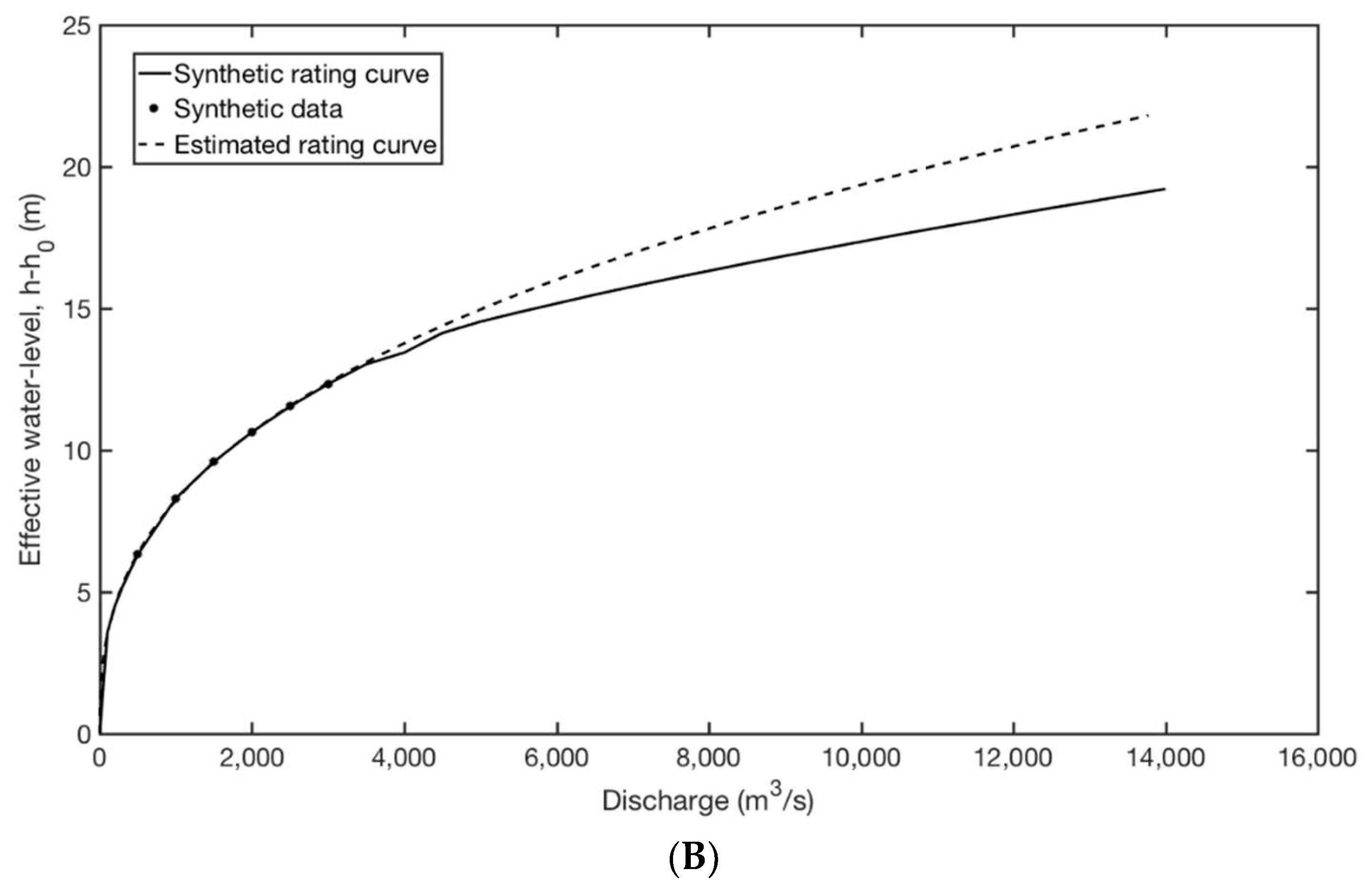
To replicate the typical estimation of design flood levels using frequency analysis of the flood discharge peaks (as shown in Figure 1), it is necessary to estimate the rating curve information at any given cross-section along the river. We applied the hydraulic model to derive a number of synthetic pairs (h, Q), which were then used to parameterize the estimated rating curve equation. The synthetic rating curve was derived by simulating in HEC-RAS flows ranging from 100 m3/s to 1000 m3/s with steps of 100 m3/s, followed by simulations of discharge ranging from 1000 m3/s to 13,000 m3/s with steps of 1000 m3/s. After that, the estimated rating curve was assessed by fitting the synthetic data pairs using a power law relationship between the water level and river flow. Data pairs for the statistical fit are discharge data ranging from 1000 m3/s to 6000 m3/s (with steps of 1000 m3/s) and their corresponding stages derived from the hydraulic simulations. The power law relationship is expressed as:
where Q* is the estimated river flow, is the cease-to-flow stage, is the measured water stage, and and are calibration parameters that can be determined by the method of non-linear least squares. Once the power law relationship is established, one can extrapolate to higher flow values.
The two rating curves are shown in Figure 2 and the full circles represent the data pairs used in deriving the estimated rating curve. Figure 2 refers to two cross-sections at 58 and 68 km downstream of Cremona. Extrapolation beyond the range of measurements leads to a systematic underestimation of discharges for this particular case.
3.3. Parent Distribution
The GEV distribution, as defined by Jenkinson [42] and parameterised using a 90-year record of annual maximum flows available from a gauging station along the Po River, was assumed to be the Parent Distribution. Our justification for selecting the GEV as a parent lies with the fact that the focus is on modelling the block maxima of water levels, and the theoretical arguments from extreme value theory are considered sufficient for this task, assuming that the discharge, , follows a GEV distribution, ~GEV, ξ, α, and are the location, scale, and shape parameters, respectively. The tail behaviour of the GEV distribution is influenced by the value of the shape parameter and generally falls in three classes: The Gumbel type () is characterised by a light upper tail, the Frechet type () has a heavy upper tail, and the Weibull type has () and is bounded above. Hence, GEV encompasses three asymptotic distributions that can be selected to model the right tail of a distribution and as such is a grand-parent.
3.4. Probability Model
The Gumbel distribution was selected as the Probability Model to fit samples drawn from the parent distribution. The Gumbel distribution is quite popular among engineering practitioners for most parts of the world. For instance, it is the distribution of choice to describe flood probabilities at the Tiber River in Rome, Italy [43].
As such, we aim to mimic the common situation in the real world, in which simple models (the Gumbel distribution in our example application) are used to fit reality (the GEV distribution in our example application). Previous studies in statistical hydrology used similar research methods, by using other simple distribution functions, such as the Lognormal, as a probability model and more complex distribution functions, such as the Kappa and Wakeby, as parent distributions [22,24].
The GEV and Gumbel quantile function is given as
where represents a quantile estimate (for either discharge or water stage) corresponding to a certain return period, in this case 100 years, while is the non-exceedance probability. The parameters of the GEV were estimated by the method of maximum likelihood using the available 90 year record of annual maximum flows. These parameters were fixed and used for generating synthetic annual maximum flows by random sampling from its inverse cumulative distribution function. Equation (2) for the condition of , which is the quantile function for GEV, was used to estimate the 100-year design peak flow. The 100-year peak flow was simulated using HEC-RAS to get the estimated design flood level,
3.5. Application of the Simulation Framework
Based on the hydraulic model (Section 3.1), rating curve (Section 3.2), parent distribution (Section 3.3), and probability model (Section 3.5), we applied our simulation framework (Section 2) to the 98-km reach of the Po River and by using a return period of 100 years (T = 100), repeating steps C–G for 1000 times (N = 1000), and exploring the role of sample size by using M equal to 30, 50, and 100. A generated sample size of 30 and 50 years reflects the typical length of historical observations, while samples of a length equal to 100 years represent an optimistic case in hydrology.
4. Results
The application of the simulation framework described in Section 2 and depicted in Figure 1, to a 98-km reach of the Po River (Section 3), allows us to compare the accuracy and precision of the two approaches for the estimation of design flood levels.
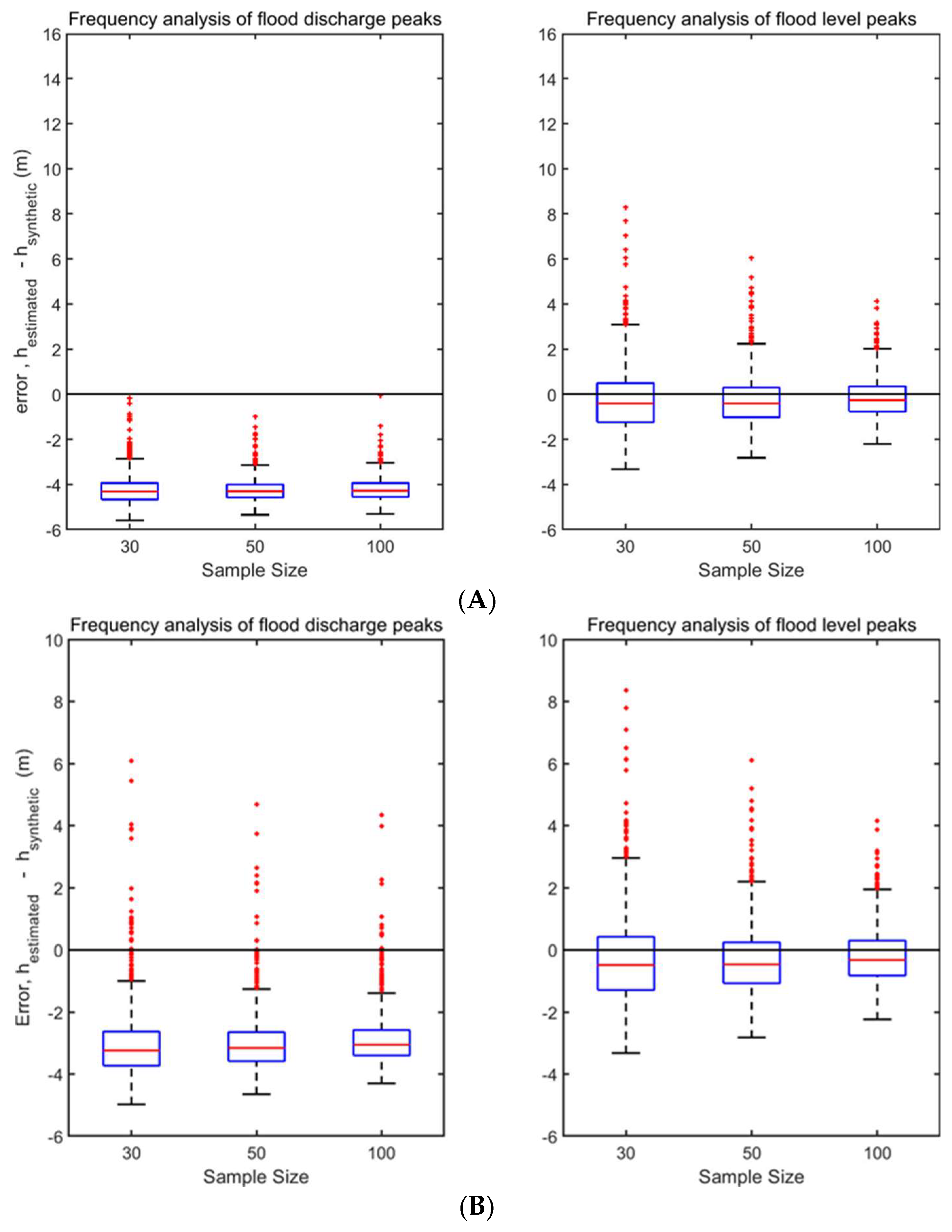
Figure 3 shows boxplots of errors when the estimation of design flood levels is based on the two methods that are considered in this study.
The left panel of Figure 3 refers to the common approach (when the estimation is based on annual maximum flows), and it shows a substantial underestimation, which is larger in section A, where the rating curve has larger errors (Figure 2). Moreover, and there is no substantial improvement in accuracy and precision after increasing the sample size from 30 to 100 years.
The right panel of Figure 3 refers to the alternative approach (when the estimation is based on annual maximum levels), and it shows an underestimation of the design flood by 0.8 m with a more significant reduction of uncertainty after increasing the sample size from 30 to 100 years. These differences are substantial when the estimation of design flood levels is used for flood defence design or risk assessment.
5. Discussion
Our results demonstrate that the alternative approach can provide lower errors in assessing the design flood level. The main advantage of the alternative approach is that less sources of uncertainty come into play, such as the ones related to rating curve estimation and hydraulic modelling structure and calibration [44,45]. In addition, the alternative approach can be easily implemented due to the low data requirement, no dependency on hydraulic modelling, and computational power. Moreover, one advantage in using high water levels is that information regarding the water stage is in abundance, or at least it can be, given the relative ease of measuring it. Also, remote sensing using satellite altimetry provides the opportunity to derive water stage data. Some studies have explored the direct use of water levels (instead of river flows) in the study of ungauged catchments [46]. Studies focusing on low flows, especially in large rivers, cannot be investigated using the alternative approach because of hydraulic sensitivity at the section control [47].
Yet, conducting flood frequency analysis using water stages is not devoid of uncertainty. For rivers with a gentle slope, water stages are heavily influenced by the downstream control (i.e., hydraulic works, roughness, channel outfall), which might lead to backwater effects and in turn affect the accuracy of the observed annual maximum water stage data. Water levels are also affected by backwater effects and hydraulic jumps forming at the gauging station [47]. Seasonal variation in channel hydraulic roughness affects the accuracy of observed water stages for a given discharge. Hence, the estimation of design flood levels based on records of water levels seems to have more potential for rivers with a subcritical flow regime and with a stable channel geometry. Di Baldassarre and Claps [12], for example, showed that flood water levels in the study area considered here (i.e., Po River) are not significantly influenced by changes in river geometry.
Moreover, while the design of levees only requires the estimation of a water level with a given return period, the design of flood control reservoirs requires an estimation of the volume of water corresponding to a given return period. In such a case, the analysis of flood discharges is needed. Furthermore, using flood discharges has other advantages, including the possibility to follow regional methods for design flood estimation, i.e., trading space for time and using multiple sites within a homogeneous region [48]. On the other hand, however, hydrogeomorphic approaches can help identify flood water levels in ungauged areas [49]. Table 1 summarizes the main advantages and disadvantage of the two approaches.
6. Conclusions
This paper presents a simulation framework (Figure 1) to compare two approaches for the estimation of design flood levels: (i) A common one based on the frequency analysis of annual maximum flows, and (ii) an alternative one based on the frequency analysis of annual maximum water levels. We proposed a virtual experiment based on the use of synthetic data to gain insights about potentials and limitations of these approaches.
The example application demonstrates that the alternative approach can work better than the common approach in terms of both accuracy and precision (Figure 3). These results were unavoidable as they were associated with the specific test site, as well as the arbitrary assumptions about the parent distribution and the hydraulic model. Still, they show that there is potential in this alternative approach, which is essentially based on very old methods of estimating potential flood levels along rivers in the past. This result is only partly surprising. While the use of annual maximum flows remains theoretically more appropriate in the context of river flooding, this approach is affected by numerous sources of uncertainty due to the use of a cascade of three models (Figure 1). As such, we suggest complementing the common approach with an alternative estimation of design flood levels directly based on annual maximum water levels, which are often the only type of data derived from direct (and typically accurate) measurements.
Our work is an initial effort to compare common and alternative approaches for the estimation of design flood levels, which we see as complementary given their corresponding pros and cons (Table 1). The simulation framework presented here can be applied elsewhere considering more parent/probability distribution functions, as well as data from various hydrogeomorphic conditions. As such, it offers new opportunities to gain more understanding about the potentials and limitations of these two alternative approaches.
Author Contributions
K.O., writing—original draft preparation; G.D.B., M.M. and K.B., writing—review and editing; K.O., Investigation; K.O., data curation; K.B., M.M. and G.D.B., supervision.
Funding
This research received no external funding.
Acknowledgments
We thank Alberto Montanari and Richard Vogel for nice discussions on previous versions of our work. Two Anonymous Reviewers are also acknowledged for constructive comments to this paper.
Conflicts of Interest
The authors declare no conflict of interest.
References
- Apel, H.; Thieken, A.; Merz, B.; Blöschl, G. Flood risk assessment and associated uncertainty. Nat. Hazards Earth Syst. Sci. 2004, 4, 295–308. [Google Scholar] [CrossRef] [Green Version]
- Merz, B.; Thieken, A.H. Separating natural and epistemic uncertainty in flood frequency analysis. J. Hydrol. 2005, 309, 114–132. [Google Scholar] [CrossRef]
- Aldrete, G.S. Floods of the Tiber in Ancient Rome; Johns Hopkins University Press: Baltimore, MD, USA, 2007. [Google Scholar]
- Di Baldassarre, G.; Saccà, S.; Aronica, G.T.; Grimaldi, S.; Ciullio, A.; Crisci, M. Human-flood interactions in Rome over the past 150 years. Adv. Geosci. 2017, 44, 9–13. [Google Scholar] [CrossRef] [Green Version]
- Angelakis, A.N.; Mays, L.W.; Koutsoyiannis, D.; Mammassis, N. Evolution of Water Supply through the Millenia: A short overview. In The Evolution of Water Supply throughout the Millennia; IWA: London, UK, 2012; pp. 553–558. [Google Scholar]
- Brandimarte, L.; Di Baldassarre, G. Uncertainty in design flood profiles derived by hydraulic modelling. Hydrol. Res. 2012, 43, 753. [Google Scholar] [CrossRef]
- Di Baldassarre, G.; Montanari, A. Uncertainty in river discharge observations: A quantitative analysis. Hydrol. Earth Syst. Sci. Discuss. 2009, 6, 39–61. [Google Scholar] [CrossRef]
- Pelletier, P.M. Uncertainties in the single determination of river discharge: A literature review. Can. J. Civ. Eng. 1988, 15, 834–850. [Google Scholar] [CrossRef]
- European ISO EN Rule 748, Measurement of Liquid Flow in Open Channels-Velocity-Area Methods; Reference Number ISO 748:1997 (E); International Standard: Geneva, Switzerland, 1997.
- Herschy, R.W. The magnitude of errors at flow measurement stations 1970. In Proceedings of the Koblenz Symposium on Hydrometry; UNESCO: Paris, France, 1973; pp. 109–131. Available online: http://hydrologie.org/redbooks/a099/099013.pdf (accessed on 5 April 2019).
- Schmidt, A.R. Analysis of Stage-Discharge Relations for Open Channel Flow and Their Associated Uncertainties. Ph.D. Thesis, University of Illionois, Champaign, IL, USA, 2004; p. 328. [Google Scholar]
- Di Baldassarre, G.; Claps, P. A hydraulic study on the applicability of flood rating curves. Hydrol. Res. 2010, 42, 10. [Google Scholar] [CrossRef]
- Aronica, G.T.; Candela, A.; Viola, F.; Cannarozzo, M. Influence of rating curve uncertainty on daily rainfall-runoff model predictions. IAHS Publ. 2006, 303, 116. [Google Scholar]
- Herschy, R.W. Hydrometry: Principles and Practice, 2nd ed.; John Wiley & Sons: New York, NY, USA, 1999. [Google Scholar]
- Petersen-Øverleir, A. Accounting for heteroscedasticity in rating curve estimates. J. Hydrol. 2004, 292, 173–181. [Google Scholar] [CrossRef]
- Potter, K.W.; Walker, J.F. An Empirical Study of Flood Measurement Error. Water Resour. Res. 1985, 21, 403–406. [Google Scholar] [CrossRef]
- Rosso, R. A linear approach to the influence of discharge measurement error on flood estimates. Hydrol. Sci. J. 1985, 30, 137–149. [Google Scholar] [CrossRef] [Green Version]
- Klemeš, V. Dilettantism in hydrology: Transition or destiny? Water Resour. Res. 1986, 22, 177S–188S. [Google Scholar] [CrossRef]
- Kuczera, G. Uncorrelated Measurement Error in Flood Frequency Inference. Water Resour. Res. 1992, 28, 183–188. [Google Scholar] [CrossRef]
- Kuczera, G. Correlated rating curve error in flood frequency inference. Water Resour. Res. 1996, 32, 2119–2127. [Google Scholar] [CrossRef]
- Kuczera, G. Comprehensive at-site flood frequency analysis using Monte Carlo Bayesian inference. Water Resour. Res. 1999, 35, 1551–1557. [Google Scholar] [CrossRef] [Green Version]
- Okoli, K.; Breinl, K.; Brandimarte, L.; Botto, A.; Volpi, E.; Di Baldassarre, G. Model averaging versus model selection: Estimating design floods with uncertain river flow data. Hydrol. Sci. J. 2018, 63, 1913–1926. [Google Scholar] [CrossRef]
- Merz, R.; Blöschl, G. Flood frequency hydrology: 1. Temporal, spatial, and causal expansion of information. Water Resour. Res. 2008, 44, 1–17. [Google Scholar] [CrossRef]
- Di Baldassarre, G.; Laio, F.; Montanari, A. Design flood estimation using model selection criteria. Phys. Chem. EarthParts A/B/C 2009, 34, 606–611. [Google Scholar] [CrossRef]
- Laio, F.; Di Baldassarre, G.; Montanari, A. Model selection techniques for the frequency analysis of hydrological extremes. Water Resour. Res. 2009, 45, W07416. [Google Scholar] [CrossRef]
- Madsen, H.; Pearson, C.P.; Rosbjerg, D. Comparison of annual maximum series and partial duration series methods for modeling extreme hydrologic events 2. Regional modeling. Water Resour. Res. 1997, 33, 759–769. [Google Scholar] [CrossRef]
- Aronica, G.; Hankin, B.; Beven, K. Uncertainty and equifinality in calibrating distributed roughness coefficients in a flood propagation model with limited data. Adv. Water Resour. 1998, 22, 349–365. [Google Scholar] [CrossRef]
- Aronica, G.; Bates, P.D.; Horritt, M.S. Assessing the uncertainty in distributed model predictions using observed binary pattern information within GLUE. Hydrol. Process. 2002, 16, 2001–2016. [Google Scholar] [CrossRef]
- Bates, P.D. Integrating remote sensing data with flood inundation models: How far have we got? Hydrol. Process. 2012, 26, 2515–2521. [Google Scholar] [CrossRef]
- Horritt, M.S.; Di Baldassarre, G.; Bates, P.D.; Brath, A. Comparing the performance of a 2-D finite element and a 2-D finite volume model of floodplain inundation using airborne SAR imagery. Hydrol. Process. 2007, 21, 2745–2759. [Google Scholar] [CrossRef]
- Xu, S.; Huang, W. Frequency analysis for predicting 1% annual maximum water levels along the Florida coast, US. Hydrol. Process. 2008, 22, 4507–4518. [Google Scholar] [CrossRef]
- Chen, Y.; Huang, W.; Xu, S. Frequency Analysis of Extreme Water Levels Affected by Sea- Level Rise in East and Southeast Coasts of China. J. Coast. Res. 2014, 68, 105–112. [Google Scholar] [CrossRef]
- Razmi, A.; Golian, S.; Zahmatkesh, Z. Non-Stationary Frequency Analysis of Extreme Water Level: Application of Annual Maximum Series and Peak-over Threshold Approaches. Water Resour. Manag. 2017, 31, 2065–2083. [Google Scholar] [CrossRef]
- Fürst, J.; Bichler, A.; Konecny, F. Regional frequency analysis of extreme groundwater levels. Groundwater 2015, 53, 414–423. [Google Scholar] [CrossRef]
- Dyhouse, G.R. Stage-frequency analysis at a major river junction. J. Hydraul. Eng. 1985, 111. [Google Scholar] [CrossRef]
- HEC (Hydrologic Engineering Center). Hydraulic Reference Manual; US Army Corps of Engineers: Davis, CA, USA, 2001.
- Pappenberger, F.; Beven, K.; Horritt, M.; Blazkova, S. Uncertainty in the calibration of effective roughness parameters in HEC-RAS using inundation and downstream level observations. J. Hydrol. 2005, 302, 46–69. [Google Scholar] [CrossRef]
- Pappenberger, F.; Matgen, P.; Beven, K.J.; Henry, J.B.; Pfister, L.; Fraipont, P. Influence of uncertain boundary conditions and model structure on flood inundation predictions. Adv. Water Resour. 2006, 29, 1430–1449. [Google Scholar] [CrossRef]
- Schumann, G.; Member, S.; Hostache, R.; Puech, C.; Hoffmann, L.; Matgen, P.; Pfister, L. High-Resolution 3-D Flood Information From Radar Imagery for Flood Hazard Management. IEEE Trans. Geosci. Remote Sens. 2007, 45, 1715–1725. [Google Scholar] [CrossRef]
- Brandimarte, L.; Brath, A.; Castellarin, A.; Di Baldassarre, G. Isla Hispaniola: A transboundary flood risk mitigation plan. J. Phys. Chem. Earth 2009, 34, 209–218. [Google Scholar] [CrossRef]
- Di Baldassarre, G.; Castellarin, A.; Brath, A. Analysis of the effects of levee heightening on flood propagation: Example of the River Po, Italy. Hydrol. Sci. J. 2009, 54, 1007–1017. [Google Scholar] [CrossRef]
- Jenkinson, A.F. The frequency distribution of the annual maximum (or minimum) values of meteorological elements. Q. J. R. Meteorol. Soc. 1955, 81, 158–171. [Google Scholar] [CrossRef]
- Calenda, G.; Mancini, C.P.; Volpi, E. Distribution of the extreme peak floods of the Tiber River from the XV century. Adv. Water Resour. 2005, 28, 615–625. [Google Scholar] [CrossRef]
- Di Baldassarre, G.; Laio, F.; Montanari, A. Effect of observation errors on the uncertainty of design floods. Phys. Chem. Earth 2012, 42–44, 85–90. [Google Scholar] [CrossRef]
- Horner, I.; Renard, B.; Le Coz, J.; Branger, F.; Mcmillan, H.K.; Pierrefeu, G. Impact of Stage Measurement Errors on Streamflow Uncertainty. Water Resour. Res. 2018, 1952–1976. [Google Scholar] [CrossRef]
- Bjerklie, D.M.; Moller, D.; Smith, L.C.; Dingman, S.L. Estimating discharge in rivers using remotely sensed hydraulic information. J. Hydrol. 2005, 309, 191–209. [Google Scholar] [CrossRef]
- Lang, M.; Pobanz, K.; Renard, B.; Renouf, E.; Sauquet, E. Extrapolation of rating curves by hydraulic modelling, with application to flood frequency analysis. Hydrol. Sci. J. 2010, 55, 883–898. [Google Scholar] [CrossRef] [Green Version]
- Blöschl, G.; Sivapalan, M.; Savenije, H.; Wagener, T.; Viglione, A. (Eds.) Runoff Prediction in Ungauged Basins: Synthesis Across Processes, Places and Scales; Cambridge University Press: Cambridge, UK, 2013. [Google Scholar]
- Nardi, F.; Annis, A.; Di Baldassarre, G.; Vivoni, E.R.; Grimaldi, S. GFPLAIN250m, a global high-resolution dataset of Earth’s floodplains. Sci. Data 2019, 6, 180309. [Google Scholar] [CrossRef]
Figure 1.
Virtual experiment proposed in this study. Graphical representation of the simulation framework to compare the estimation of design flood levels based on two alternative approaches.
Figure 1.
Virtual experiment proposed in this study. Graphical representation of the simulation framework to compare the estimation of design flood levels based on two alternative approaches.

Figure 2.
Synthetic and estimated rating curves derived using the Hydrologic Engineering Center’s River Analysis System (HEC-RAS) model and the power law models for two cross-sections located 58 km (A) and 68 km (B) downstream of Cremona (Po River, Italy).
Figure 2.
Synthetic and estimated rating curves derived using the Hydrologic Engineering Center’s River Analysis System (HEC-RAS) model and the power law models for two cross-sections located 58 km (A) and 68 km (B) downstream of Cremona (Po River, Italy).


Figure 3.
Boxplots of error estimates for the two approaches with Gumbel distribution used for design flood level estimation at cross-sections (A,B). The red lines represent the median (50th percentile), the lower and upper ends of the blue box represent the 25th and 75th percentile, respectively. Outliers are represented by red dots.


Table 1.
Summary of pros (+) and cons (−) of the two approaches.
| Various Aspects and Applications | Common Approach (Flood Discharges) | Alternative Approach (Flood Levels) |
|---|---|---|
| Sources of uncertainty | − | + |
| Computational time | − | + |
| Data requirement | − | + |
| Changes in the river channel (e.g., erosion) | + | − |
| Hydraulic effects on the channel (e.g., backwater) | + | − |
| Design of levees | − | + |
| Design of flood-control reservoirs | + | − |
| Regionalization methods | + | − |
| Hydrogeomorphic methods | − | + |
© 2019 by the authors. Licensee MDPI, Basel, Switzerland. This article is an open access article distributed under the terms and conditions of the Creative Commons Attribution (CC BY) license (http://creativecommons.org/licenses/by/4.0/).
Share and Cite
MDPI and ACS Style
Okoli, K.; Breinl, K.; Mazzoleni, M.; Di Baldassarre, G. Design Flood Estimation: Exploring the Potentials and Limitations of Two Alternative Approaches. Water 2019, 11, 729. https://doi.org/10.3390/w11040729
AMA Style
Okoli K, Breinl K, Mazzoleni M, Di Baldassarre G. Design Flood Estimation: Exploring the Potentials and Limitations of Two Alternative Approaches. Water. 2019; 11(4):729. https://doi.org/10.3390/w11040729
Chicago/Turabian StyleOkoli, Kenechukwu, Korbinian Breinl, Maurizio Mazzoleni, and Giuliano Di Baldassarre. 2019. "Design Flood Estimation: Exploring the Potentials and Limitations of Two Alternative Approaches" Water 11, no. 4: 729. https://doi.org/10.3390/w11040729
Note that from the first issue of 2016, this journal uses article numbers instead of page numbers. See further details here.