FLIAT, An Object-Relational GIS Tool for Flood Impact Assessment in Flanders, Belgium
by
 ,
,
Samuel Van Ackere
1,* ,
,
Jochem Beullens
1,
Wouter Vanneuville
2,
Alain De Wulf
1 and
Philippe De Maeyer
1
1
Department of Geography, Ghent University, 9000 Ghent, Belgium
2
European Environment Agency, 1050 Copenhagen, Denmark
*
Author to whom correspondence should be addressed.
Water 2019, 11(4), 711; https://doi.org/10.3390/w11040711
Submission received: 11 February 2019
/
Revised: 8 March 2019
/
Accepted: 10 March 2019
/
Published: 6 April 2019
(This article belongs to the Section Urban Water Management)
Abstract
:Floods can cause damage to transportation and energy infrastructure, disrupt the delivery of services, and take a toll on public health, sometimes even causing significant loss of life. Although scientists widely stress the compelling need for resilience against extreme events under a changing climate, tools for dealing with expected hazards lag behind. Not only does the socio-economic, ecologic and cultural impact of floods need to be considered, but the potential disruption of a society with regard to priority adaptation guidelines, measures, and policy recommendations need to be considered as well. The main downfall of current impact assessment tools is the raster approach that cannot effectively handle multiple metadata of vital infrastructures, crucial buildings, and vulnerable land use (among other challenges). We have developed a powerful cross-platform flood impact assessment tool (FLIAT) that uses a vector approach linked to a relational database using open source program languages, which can perform parallel computation. As a result, FLIAT can manage multiple detailed datasets, whereby there is no loss of geometrical information. This paper describes the development of FLIAT and the performance of this tool.
1. Introduction
Worldwide, floods cause over one-third of overall economic losses due to natural hazards. These losses are particularly severe in urban environments. Moreover, the severity and frequency of floods are expected to increase over the 21st century [1]. Therefore, there is a compelling need for resilience against extreme events, such as floods. To mitigate these extreme events, priority adaptation guidelines, measures, and policy recommendations must clearly indicate what can be done to adapt to natural hazards linked to climate change. Most settlements are not adapted to inundations [2], and because they are often located close to rivers or coastlines, valuable and vulnerable land uses are exposed to floods. Due to urban developments in floodplains, space for the rivers shrinks and water levels increase [3].
Traditionally, floods have been controlled with artificial, engineered infrastructures (i.e., dykes and dams) [4]. Rather than attempting to preserve the existing urban structure, however, more flexible measures are sometimes required in which adaptive cities are revamped by (the threat of) flood events [3]. Combining flood adaptation measures with public space design can serve multiple purposes, including water depuration, recreation, or microclimatic melioration [5]. Natural water retention measures (NWRMs) and ecosystem-based adaptations, including green roofs, development of buffer zones, rain gardens, and the deployment of rainwater wells and barrels (e.g., using rainwater for washing machines, toilets, maintenance), can be employed in urban residential areas [6,7,8,9].
Nonetheless, these priority adaptation guidelines can also provide technical measures, e.g., inserting gates where needed, building sluices to prevent ingress of water into drains, raising floor levels in vulnerable town centre properties, installing breakwaters, implementing self-closing barriers at underground car parks, etc.
To determine the balance between these flexible and robust measures and where these measures need to be applied, first, a priority adaptation (road) map is needed.
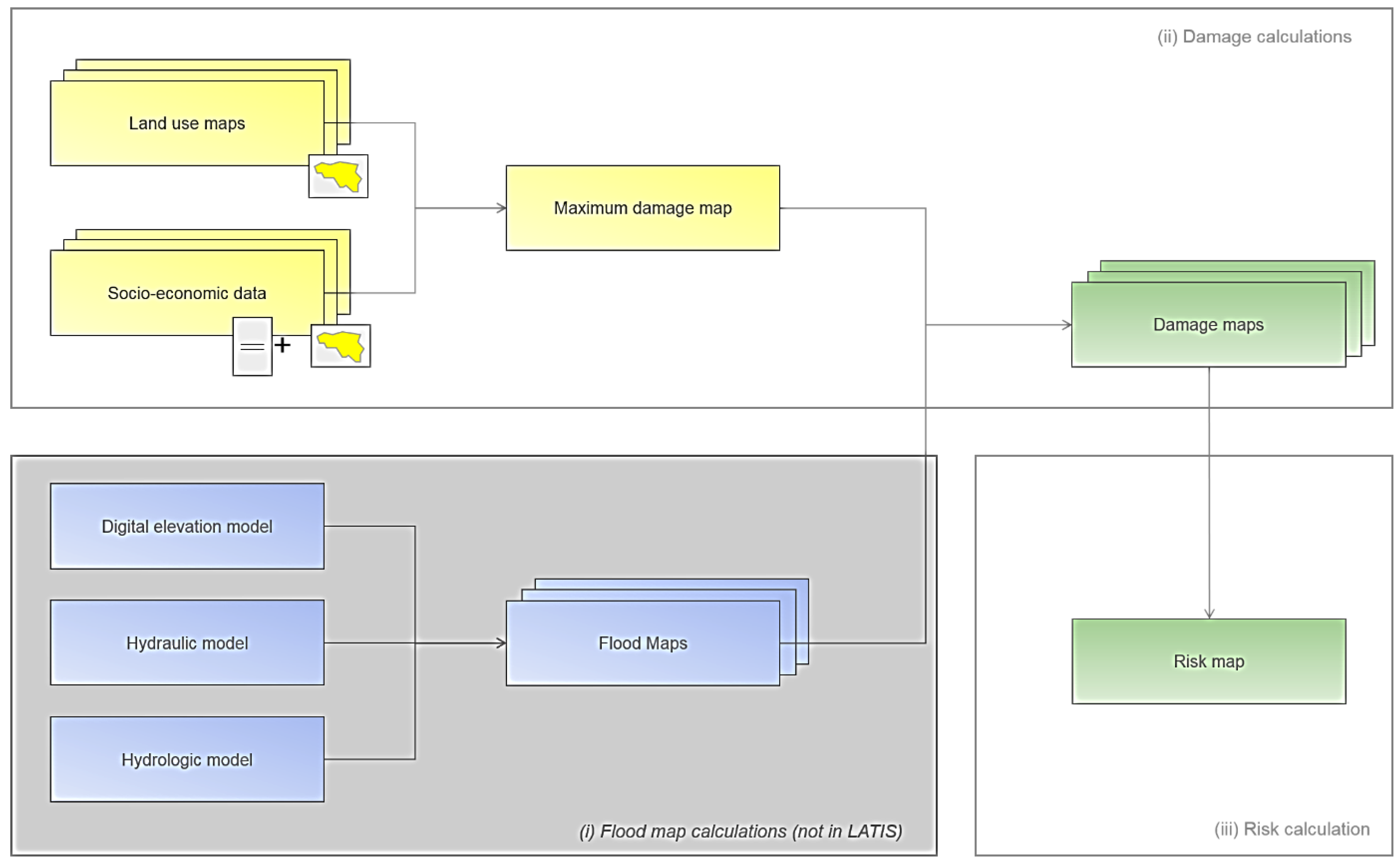
Since 2002, Ghent University, in collaboration with Flanders Hydraulics Research, developed a methodology that computes the socio-economic impact of floods, which is determined based on land use information, socio-economic data, and damage functions (see Figure 1).
The economic risk and the risk for victims can be measured by considering the expected damage or number of victims for different return periods with a risk formula [10]. Through the years, the development of the social, ecologic, and cultural impact assessment was added to this existing methodology. Because of the lack of server performance and computing power back in 2003, the LATIS tool was developed with a raster approach and programmed in C#.Net that used the GIS (geographic information system) technology of IDRISI (raster-GIS) [10].
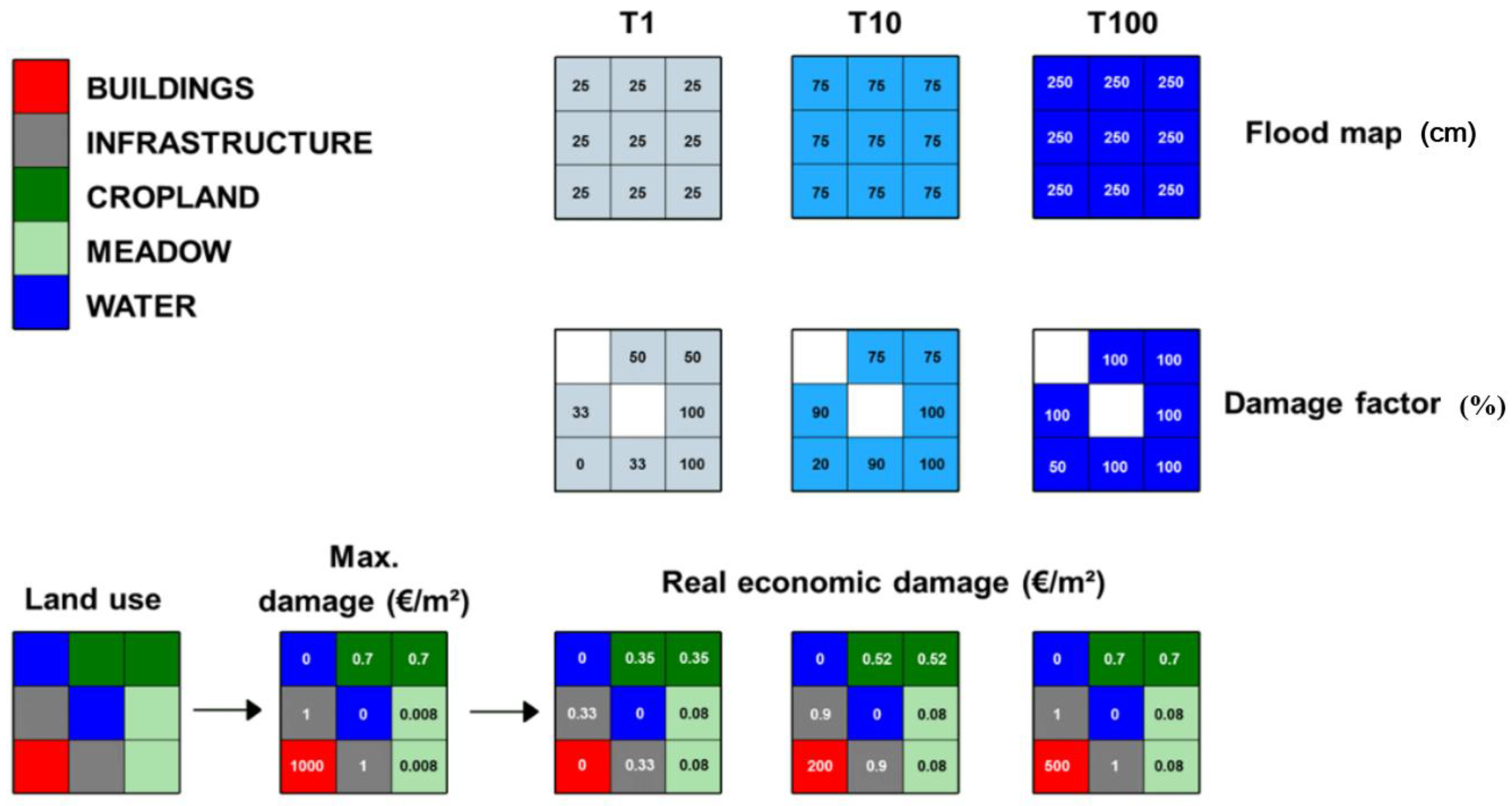
To calculate the economic damage resulting from floods with a raster approach (see Figure 2), land use data is converted in raster files in which every land use category is translated into an estimated economic replacement value (or maximum economic damage) by using the Standard Method [11].
Like the flood impact assessment tool LATIS in Flanders, Belgium, many other flood impact assessment tools use the raster approach to calculate socio-economic damage resulting from floods. For example, Delft-FIAT in the Netherlands requires raster files to run its script. Therefore, the tool comes with a free available pre-processing Python script based on the Geospatial Data Abstraction Library (GDAL) library to convert all land use and object data from vector files to raster data with the required Delft-FIAT settings [13]. A widely used variant of this tool is the HIS-SSM/SSM-2017 tool, also developed for the Netherlands [14], in which all data is standardized by converting the vector files into raster files with a resolution of 5, 25, 50, or 100 m [15]. The same applies to Flemo for Germany [16,17], HAZUS for the USA, and the CORFU tool for Europe and Asia [18,19], where all input variables are processed to be available as raster datasets with a cell size relatively equal to the water depth raster file.
To calculate the socio-economic damage, either the default source data that is included with the specific damage assessment tool (e.g., LATIS, HAZUS, etc.) can be used, or the user can choose to upload their own data that is, for example, more applicable to their assessment study (e.g., more detailed data, emphasis on other flood parameters, etc.). In reference to Flanders, the source data of the LATIS tool has a resolution of 5 m by default and can immediately be used for an assessment of a specific flood event.
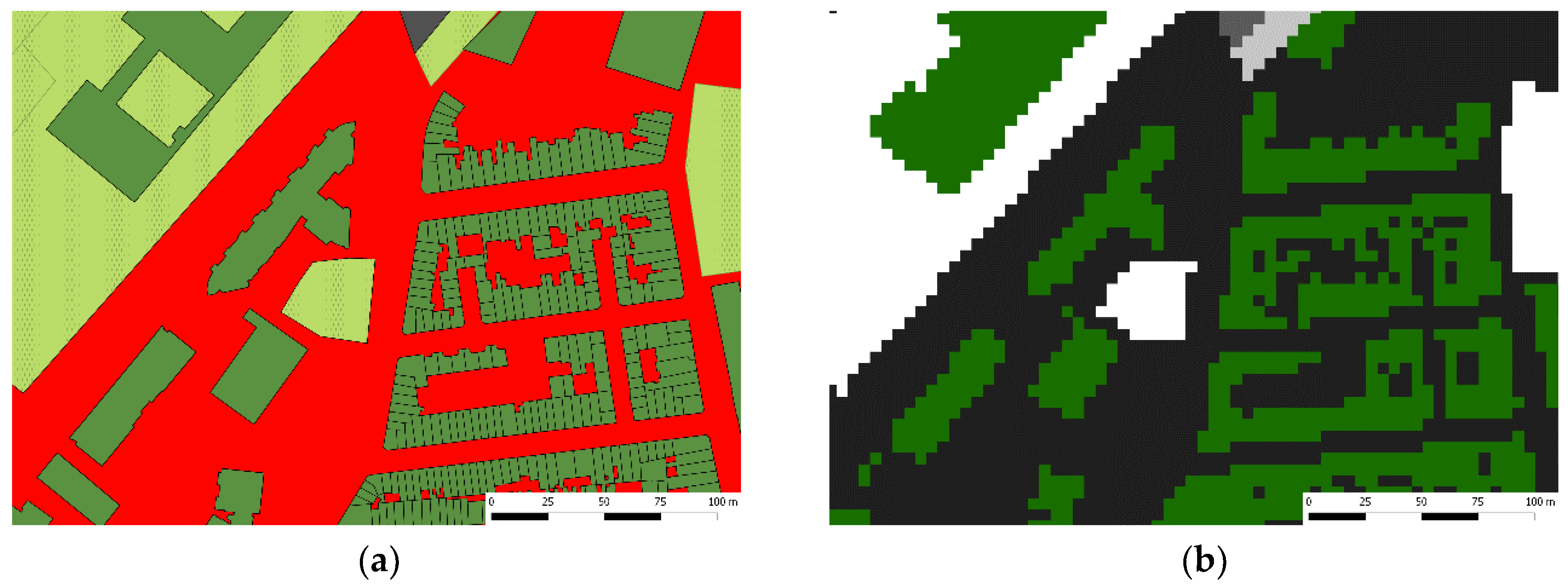
Regardless of differences in methodology, there are a number of disadvantages that come with the raster approach to flood impact assessment tools (see Figure 3). Chen et al. show that parcel areas and buildings are overestimated when they are represented by large raster cells (larger or equal than 5 m) because, in many cases, only a portion of a cell is occupied by it, while the whole cell area is used to represent this small parcel or building [19]. In fact, this spatial error applies to all land use and objects that need to be converted from vector data to raster data. Although it is possible to differentiate separate objects when the cell size is not too big, parcel boundaries do not align with the cell boundaries when polygons are converted to raster format. Smaller grid cells reduce this error but increase the computation load and the data storage requirements. Citing Bai et al., “Rasterization is a conversion process accompanied with information loss, which includes the loss of features’ shape, structure, position, attribute and so on” [20].
Additionally, a raster consists essentially of a matrix of cells (or pixels) organized into rows and columns (a grid), where each cell contains one and only one value representing information (e.g., water depth). Of course, there are a few exceptions to the rule that one grid cell in a raster can only store one value. For example, by using the FD8 algorithm [21], it allows the raster to use combinations of base-2 numbers to store multiple flow directions towards up to eight different neighbours. Nevertheless, this FD8 algorithm is mostly used in rather specialized and limited case due to its complexity. A second scenario would be to store data in the three bands of 8-bit data (the colour composites red, green, and blue) as a single value and then parse the values when the image is read. However, this limits the data from the three data sources to a narrow numerical range (integers from 0 to 255). The last scenario is to use raster formats that allow multiple bands (e.g., BIL, BSQ, BIP, TIFF, etc.). The standard procedure to combine multiple raster files is when all combined raster files still exist. Consequently, the simplest raster GIS way to store multiple values is by using multiple raster files. Yet, a key issue is storing multi-values of one and the same category with the use of raster files (e.g., when multiple companies are settled in one building). It can be concluded that there are multiple drawbacks when a flood impact assessment tool is developed with a raster approach.
Before the flood impact can be assessed, reliable and accurate flood maps are required. To date, there are many 2D depth-averaged flood simulation models (e.g., TELEMAC-2D [22], MIKE21 [23], DIVAST [24,25]). Hereby, a depth-integrated solution is considered to be sufficiently accurate in shallow water comparisons [26]. These depth-averaged tools have a wide range of applications [27,28,29,30]. Yet in floods with a significant variance in pressure over the water column, a three-dimensional model is required. Three-dimensional models (e.g., TRIVAST [29], EFDC [31], TIDE3D [32], and TELEMAC-3D [33]) also solve the Navier–Stokes set of equations [34], but work with multiple layers over the depth and can, thus, model pressure and speed gradients over the depth. These flood simulation models have been constrained by the scarcity of detailed and accurate digital elevation models (DEMs). Luckily, accuracy has improved over the years because of the emergence of new data capture techniques, particularly in the field of aerial digital photogrammetry [35] and airborne remote sensing, including interferometric synthetic aperture radar (SAR) [36] and light detection and ranging (LiDAR) [37].
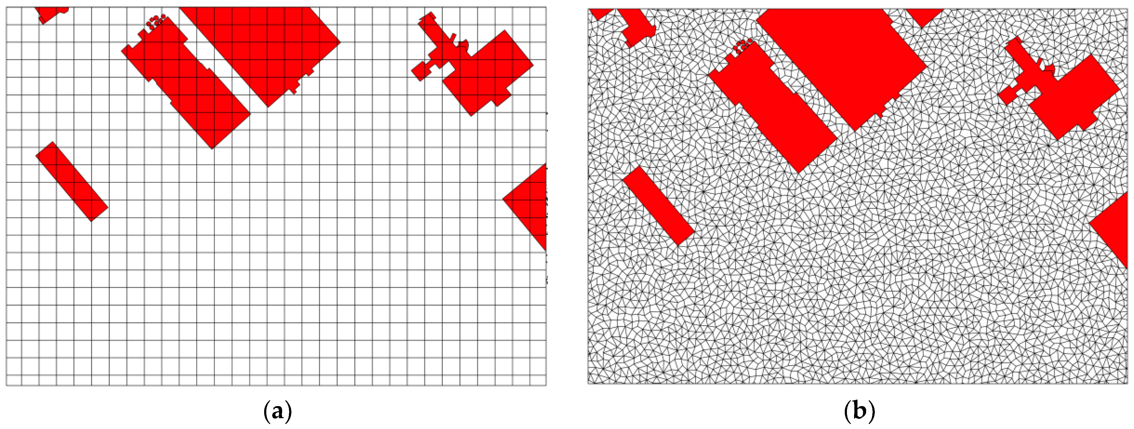
DEM can be represented as raster, TIN, or unstructured meshes (eventually with localized refinements) to calculate and simulate flood inundation [38] (see Figure 4).
A raster-based structure makes it possible to represent the complex topographical elevation as highly predefined, discrete areas [39]. The grid cell resolution indicates the size of the grid cell in which small grid cells are defined by a high resolution. DEM accuracy decreases with coarser resolutions [40]. As a result, a high resolution allows a better representation of complex topography with a greater accuracy [41]. It has been shown that a low resolution of DEM has a tremendous impact on slope algorithm calculations (the calculated maximum slope becomes larger as the DEM resolution becomes finer), as complex topographies are flattened due to its averaging [42,43,44,45]. The resolution of DEM also has a significant impact on hydraulic and hydrological modelling, such as horizontal and vertical flow direction and velocity [41,46,47], erosion and sedimentation modelling [42], catchment areas derived from DEM [46], computation of soil water content [48], etc. Even relatively small changes in DEM resolution have considerable effects on the predicted inundation extent and the timing of flood inundation [49].
Attention should be paid when raster data with a low spatial resolution is combined with raster data of a relatively much higher spatial resolution (e.g., raster data with a resolution of 1 km combined with raster data with a resolution of 10 m). The output will most likely be unidentifiable, as the scales of analysis are far too disparate to result in interpretable and/or meaningful conclusions. Therefore, it is recommended to calculate the socio-economic impact of floods on the basis of flood data with a spatial resolution that is relatively equal to the land use data.
Analogous to the impact of the resolution of raster-based DEM, the size of unstructured meshes has an enormous impact on the accuracy of hydraulic modelling [50]. The advantage of unstructured meshes is in its ability to easily vary cell size throughout the changes of the terrain in which unstructured meshes can describe the terrain more accurately than raster-based DEM with a comparable resolution [51,52]. Consequently, the unpredictable randomness of unstructured, irregular meshes makes it impossible to convert this data type into a raster file without considerable error.
Because the accuracy of the output of hydraulic simulation models is dependent on the accuracy of the input of the digital elevation model, the unstructured mesh-based hydraulic simulation model output has a greater accuracy than a raster-based hydraulic simulation model output with a comparable resolution (unless there is only a raster-based digital terrain model available). Therefore, by immediately calculating flood impact using the unstructured mesh data type instead of immediately converting the hydraulic simulation into a raster, no loss of accuracy will occur.
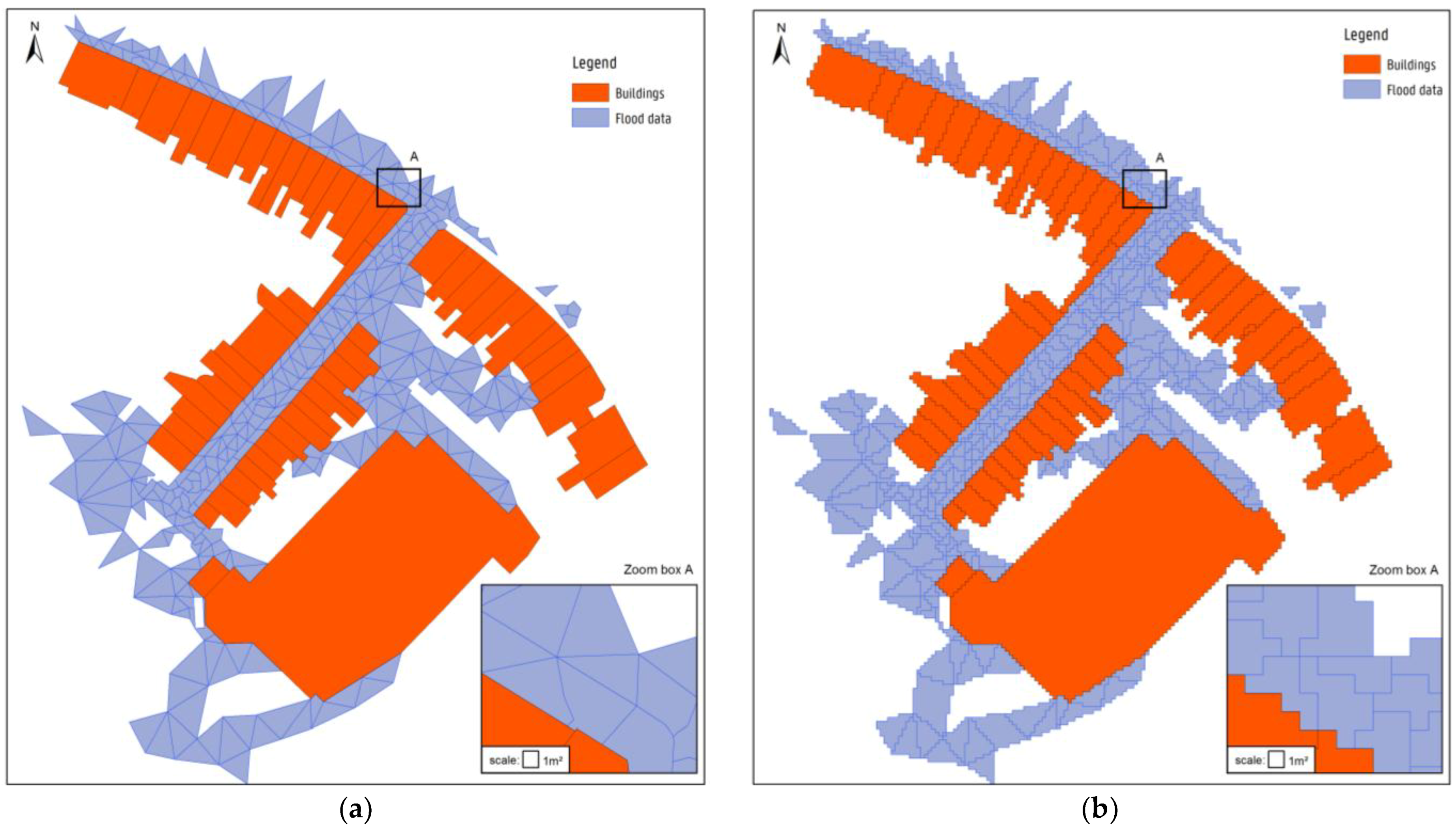
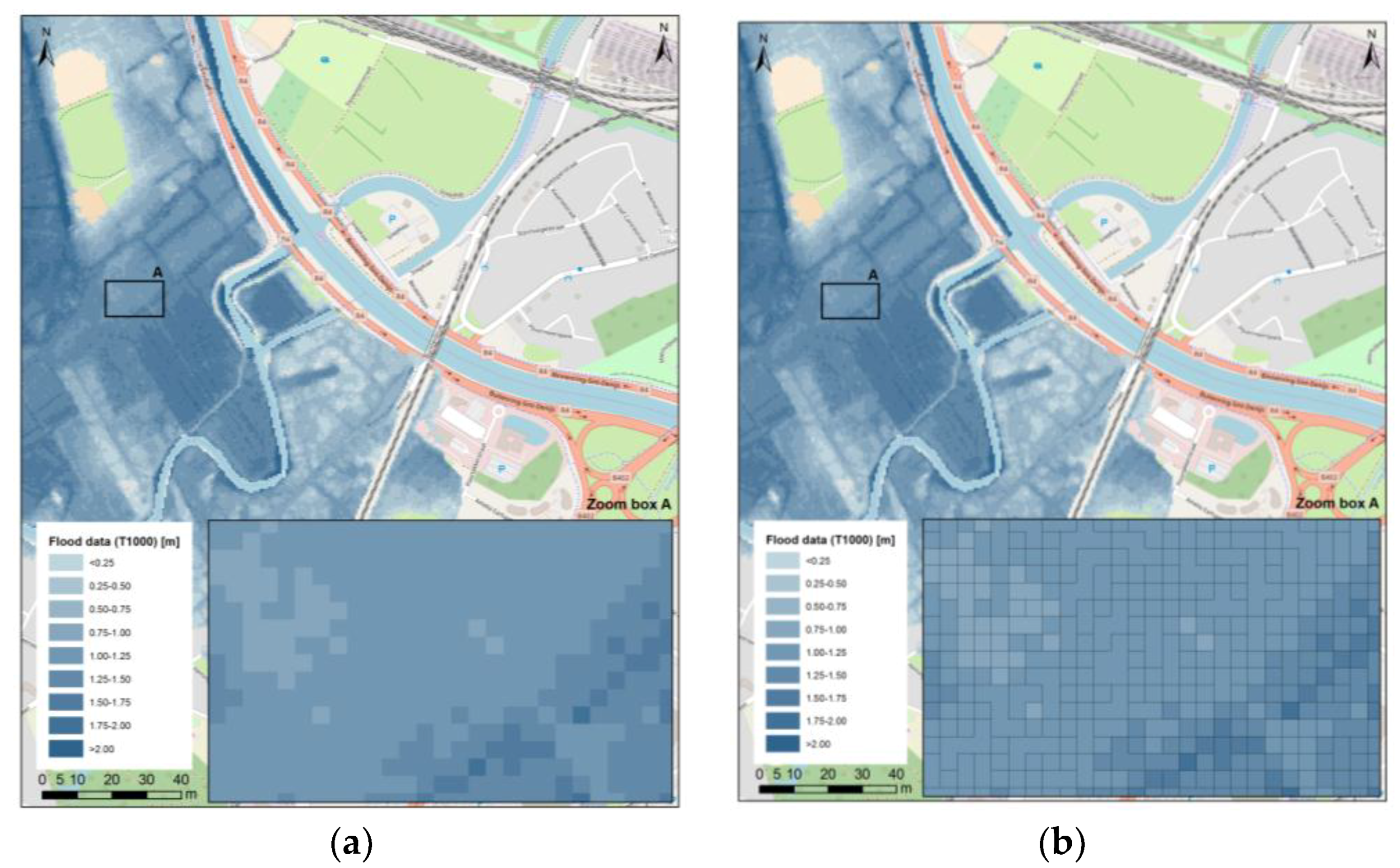
Additionally, more and more hydraulic simulation models are modelling floods by taking buildings, infrastructures, and other objects into account as obstacles for water flow instead of assuming a permeability of 100% for these objects. As a result, the flood boundaries correspond to the boundaries of the objects on the terrain (see Figure 5a). After converting these unstructured mesh-based flood data into raster-based flood data, there is no overlap of grid cells of the flood data with the object (see Figure 5b). One exception is in the unlikely case of the equal occurrence of land use (e.g., buildings) and flood data in one raster cell.
Because of this, a new flood impact assessment tool (FLIAT) is needed that can compute the impact of floods using both a vector approach and a raster approach (when needed), which can handle multiple data sets in a fluent way. Hereby, it is not necessary to run the FLIAT tool with additional data or by using more detailed data compared with the current damage assessments. Nevertheless, this FLIAT tool can be used in detailed flood impact studies, for example when a (societal) cost-benefit analysis of individual measures (or a group of measures in a limited area) is made. The FLIAT tool helps engineers, environmental agencies, and local governments accurately detect and define the priority protection zones, in terms of socio-economic damage and social disruption resulting from flood events, on the basis of the uploaded flood simulation data (or occurred flood events) of a specific region. FLIAT can be used in cost-benefit analyses of, for example, sewerage and road construction projects and the construction of (coastal) protection infrastructures, and this makes the tool valuable as a decision-making tool for priority adaptation guidelines, measures, and policy recommendations. This paper will explore a suitable methodology for calculating the impact of floods with a vector approach and describes the development of the FLIAT prototype [53]. In Section 3, case studies of a river flood and a pluvial flood in the city of Ghent and a coastal flood at the Belgian coast are worked out with the proposed FLIAT vector-based approach and the raster approach in order to compare the performance of both approaches, including running speed and accuracy.
2. Methodology
Compared to 2002 (start of development of LATIS in Flanders), there are now multiple arguments that support the feasibility of calculating the impact of floods with a vector approach. First of all, there are enhanced insights in vector calculation using R-tree [54,55] over-GiST (Generalized Search Tree) spatial indexes for high-speed spatial querying [55]. R-tree-over-GiST spatial indexes make the searching algorithms (e.g., intersection, containment, nearest neighbour search) easier, because these indexes “(…) break up data into rectangles, and sub-rectangles, and sub-sub rectangles, and so on” [55], and they decide whether or not the calculation needs to happen inside a subtree using these bounding boxes. Without the use of these indexes, any search for a feature would require a “sequential scan” of every record in the database, and a simple vector calculation algorithm would become very time-consuming.
Additionally, there is a tremendous improvement in server performance and computing power [56]. This improvement allowed for the development of parallel computation, a type of computation in which many calculations are carried out in parallel [57].
2.1. Flood Impact Assessment Tool (FLIAT) Tool
The FLIAT prototype was developed in the open source relational database system PostgreSQL, with the spatial database add-on PostGIS [58]. PostGIS is provided with an R-Tree-over-GiST scheme (since version 0.6), which can be activated with a PostgreSQL database adapter for the open source Python programming language Psycopg [59]. Because PostgreSQL/PostGIS and Python can run on various operating systems, FLIAT is a cross-platform application (e.g., Windows, OSX, Linux, etc.) and can run on various devices (e.g., desktops, laptops, servers, and high-performing infrastructures (HPC)). In addition, FLIAT can run in parallel on multiple cores, which speeds up calculation [59].
To begin, all the vector-based land use data was uploaded to the PostgreSQL/PostGIS database (e.g., buildings, roads, infrastructure, electricity infrastructure, etc.), in which each table in the PostgreSQL/PostGIS database embedded one category of land use. Each polygon that represented one specific object (e.g., building) or one specific piece of land (e.g., meadow) was saved as a hex-encoded geometry type with a unique ID and distinct values (e.g., area, the age of the building, type of building, etc.) (see Table 1).
Additionally, datasets with potential multiple data per category, such as enterprise activity code (NACE) [60] (see Table 2), the age of each inhabitant, etc., were saved in separate tables per category by linking the data with the unique ID of each land use (e.g., building). The NACE code is a code assigned by the European Union and its Member States to a certain class of economic activities (whether or not commercial). This was intended as an aid in the preparation of economic statistics and overviews.
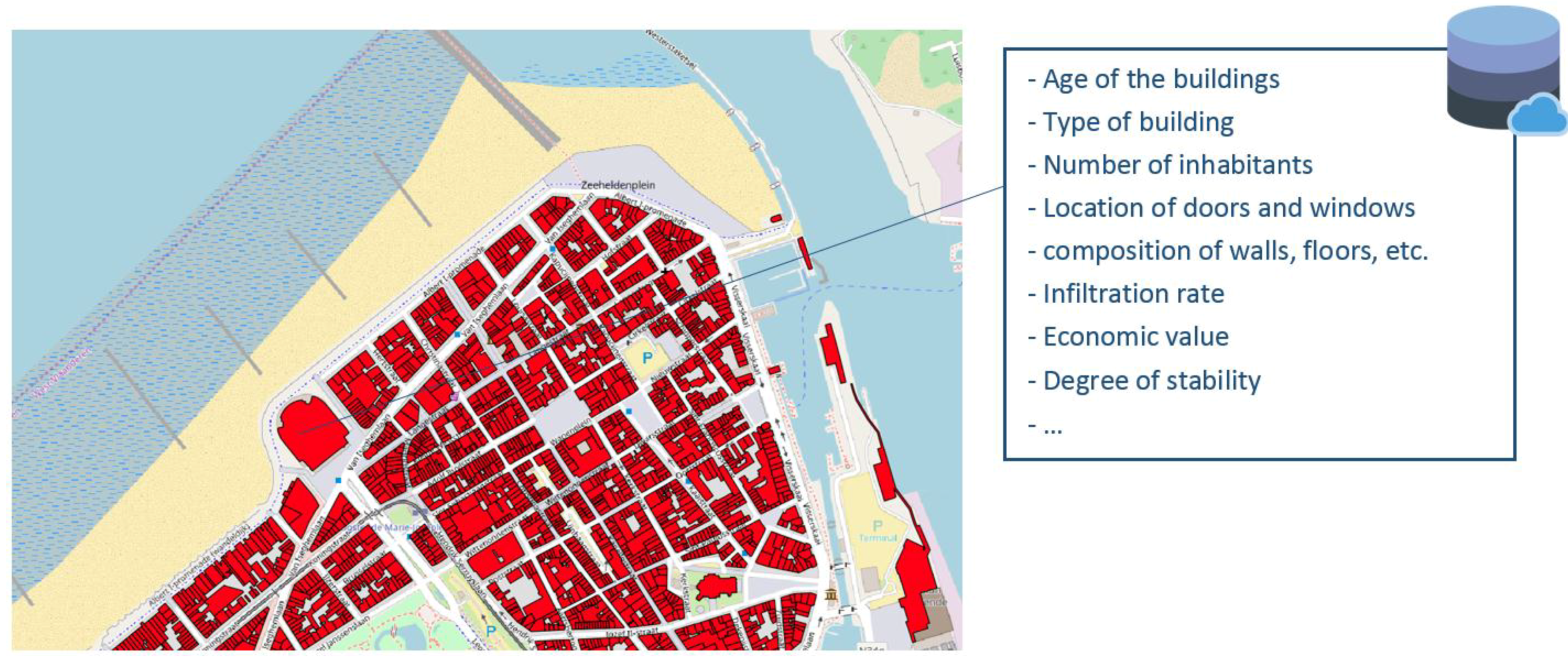
Thus, FLIAT can handle a variety of multiple detailed data sets with no loss of geometrical information (see Figure 6). It can also handle multiple datasets that are linked to well-defined elements (e.g., the detailed characterization of sluices and gates, the part of a city linked to a specific energy infrastructure, the location of doors and windows in a building, etc.) [61].
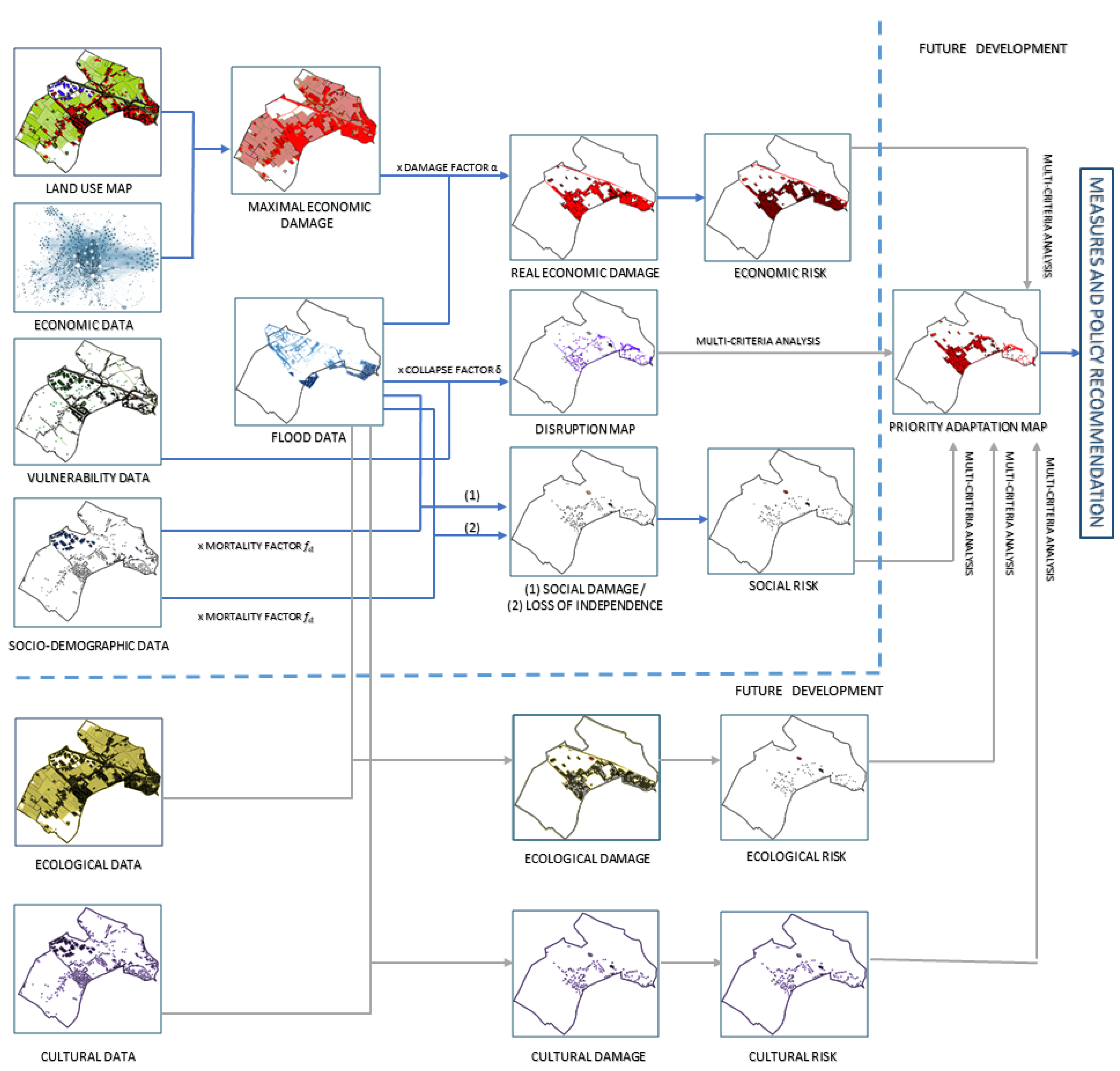
The flood impact assessment tool (FLIAT) prototype is developed to calculate the socio-economic impact of floods combined with the disruption potential analysis of a society due to these floods. In the near future, an extension of the FLIAT methodology will be developed (e.g., cultural and ecological impact assessment, and multicriteria analysis, see Figure 7 and Discussion).
2.2. Different Geographic Information System (GIS) Operations
2.2.1. Vector-based GIS operations
Because it is no longer possible to calculate the economic impact of floods with the typical raster calculation, the meshes that touch or overlay the object or land use (e.g., building, infrastructure, etc.) were taken into account to calculate the socio-economic impact (and by addition, ecologic and cultural impact in the future) of this object or land use.
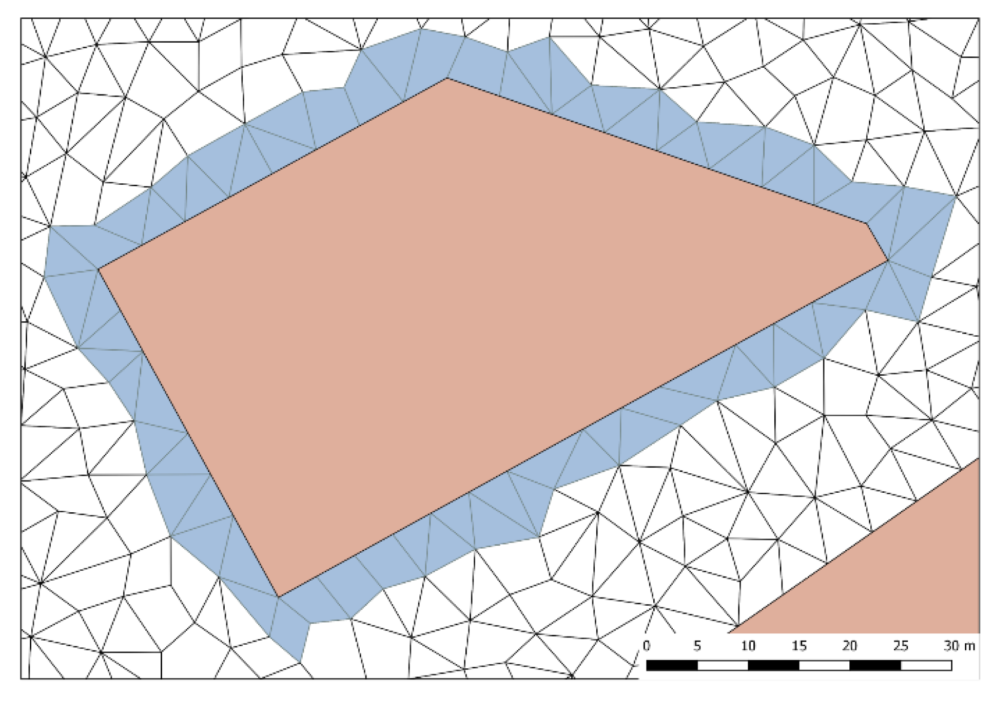
Essentially, there are two types of scenarios in which vector GIS operations are embedded in the FLIAT tool to work with vector data. In the first operation, the flood is simulated by taking objects (e.g., buildings, infrastructures, etc.) in the landscape into account as obstacles and displaying where the flood meshes touch the building (see Figure 8).
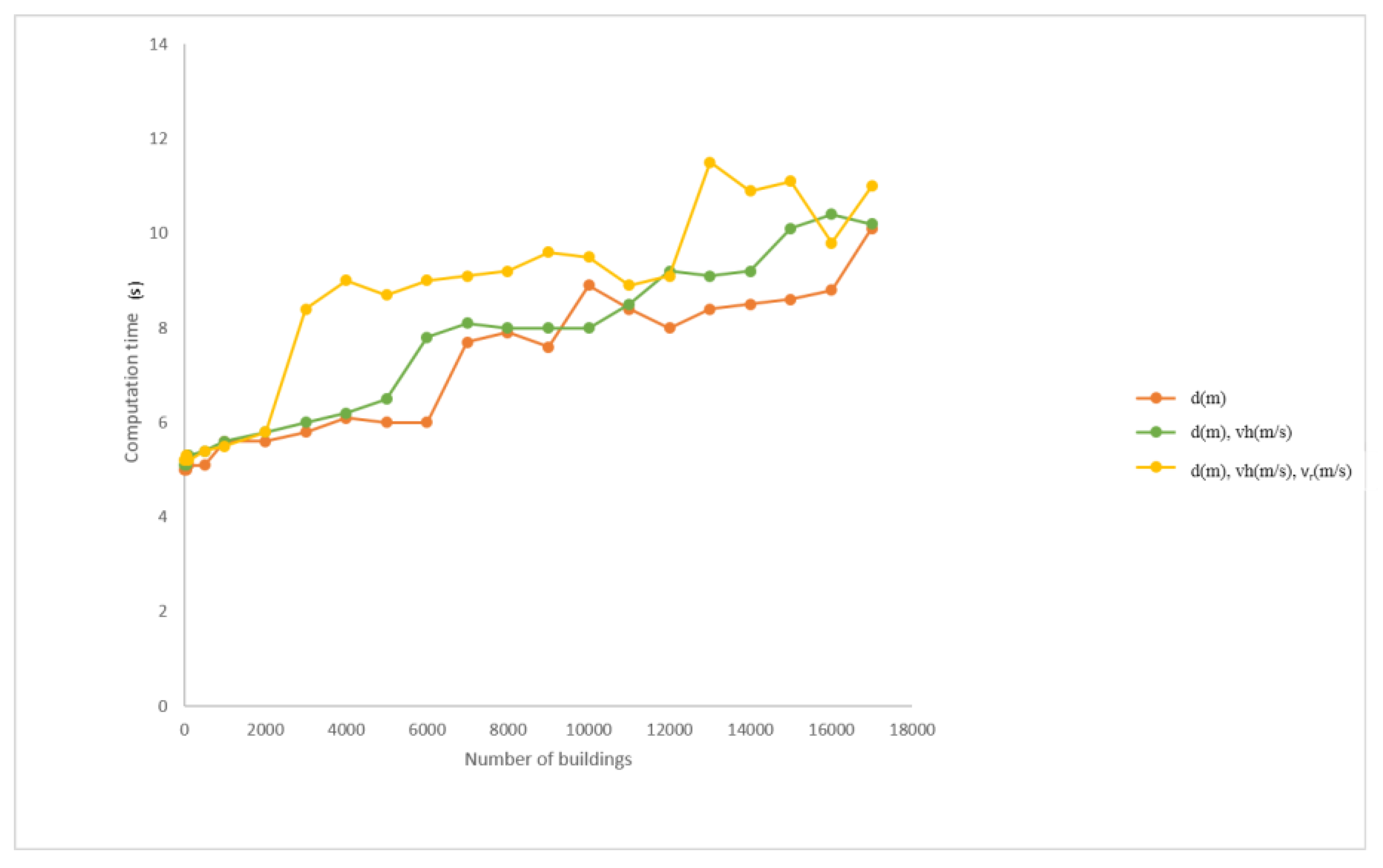
First, a temporal list of all objects that are flooded is created. Unique IDs of these objects are used to start queries that, in turn, create a temporal list with all values of the flood characteristics (e.g., water depth, horizontal and vertical flood velocity, duration, etc.) of every mesh that touches the object. Hereafter, all required values (e.g., maximal water depth, the location of maximal water depth, maximal water depth at the entrance door, maximal flood velocity, etc.) can be selected and saved to the attribute table of the object. Since the query first creates a temporal list of all values per object, and only afterwards calculates the required flood characteristics, the extra time to filter out these required values is minimal and negligible compared to the time to connect to the Postgresql/PostGIS database and create the temporal tables (see Figure 9).
Because processing time to compute the required flood characteristics is within seconds, parallel processing is not required for tens of thousands of objects. Above a larger number of objects, parallel computation can be used to speed up this process.
The second type of scenario in which a different GIS operation is embedded in the FLIAT tool is the impact calculation for flooded locations where the simulated flood event overlays the flooded land use polygons.
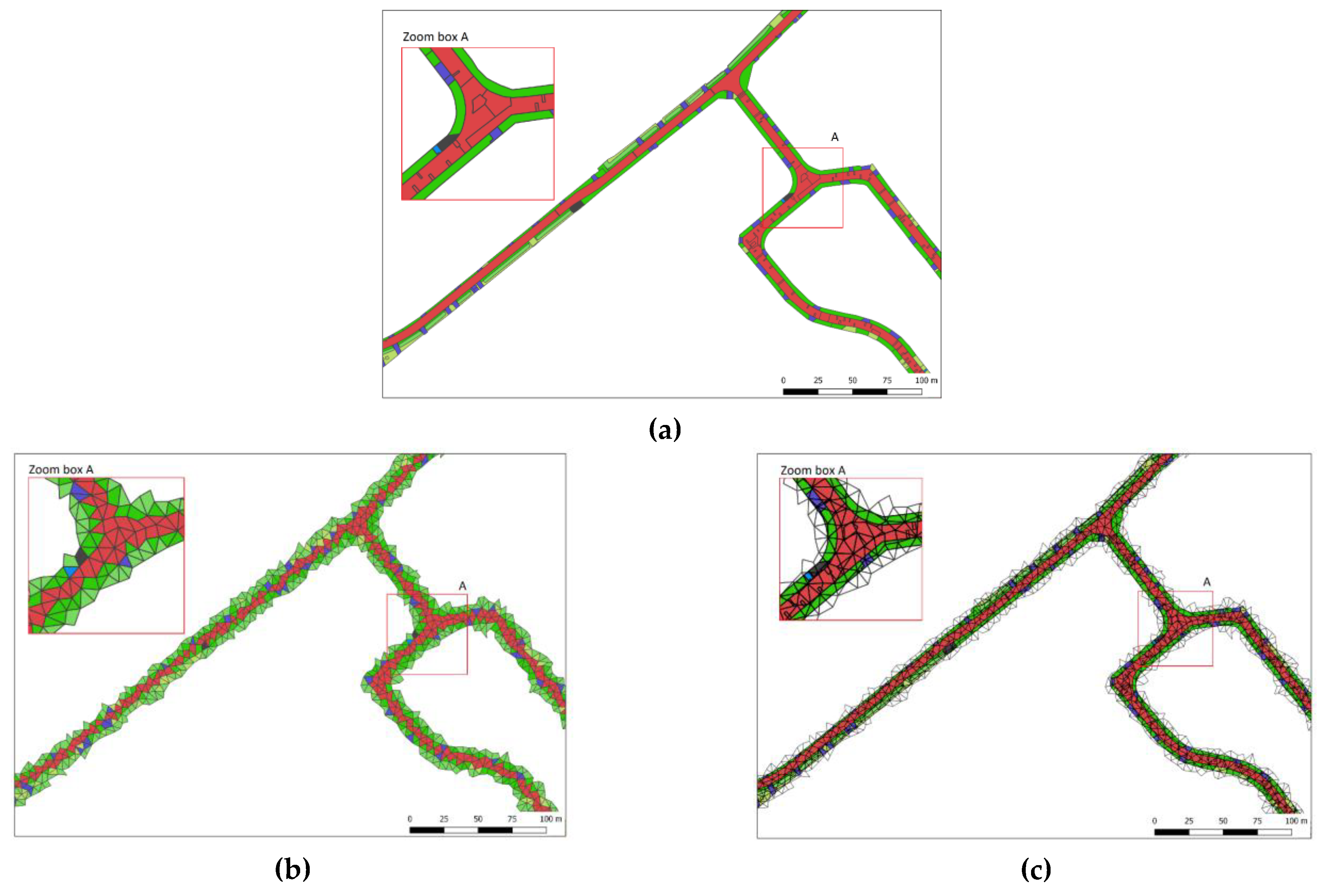
If the accuracy is less important than the computation time for the user of the FLIAT tool, the user can calculate the socio-economic impact of the flood event with FLIAT by using the mesh polygons of the flood output for the mesh-based output of the socio-economic impact (see Figure 10b). The other more detailed computation is the GIS operation, where every mesh of the unstructured mesh-based flood is split up to the lowest common denominator (see Figure 10). The output of this GIS operation still contains the detailed representation of the land use data.
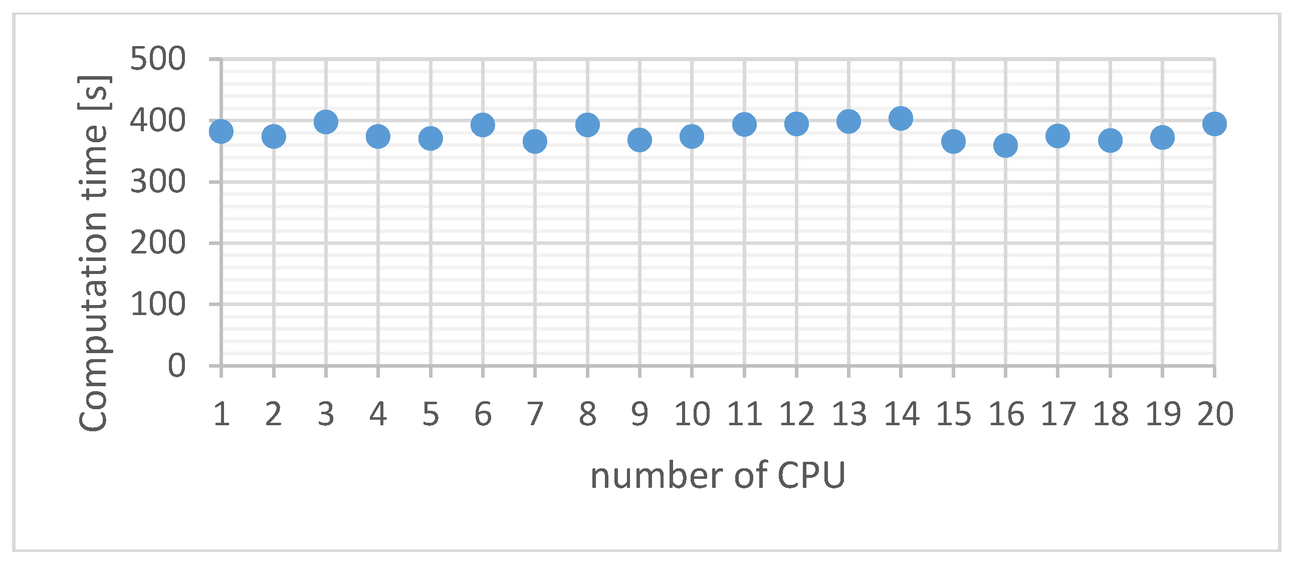
To speed up calculation of the socio-economic and, in the future, the cultural and ecological damage and risk (see Discussion), task parallelism is implemented. To optimally run this task parallelism, each task for every separate core needs to be as equal as possible, which is covered by the task distribution module in the FLIAT tool. In this way, the computation time is more or less the same for every CPU (see Figure 11).
2.2.2. Raster-based GIS Operations
In order to calculate the socio-economic impact and the disruption potential due to a flood event on the basis of raster-based flood simulation data, a conversion script comes with the FLIAT tool. This conversion script is able to convert detailed raster-based flood simulation data to polygon-based data quickly using parallel processing. First, the raster file is split into smaller units using the open source Geospatial Data Abstraction Library (GDAL) [62]. It then becomes possible to implement task parallelism and convert each unit separately to vector data on an assigned processing unit. To run this task parallelism smoothly, a multiprocessing package is used, which is part of Pathos, a Python framework for heterogeneous computing developed by Mike McKerns [63]. Each unit is converted with the open source GDAL polygonise Python script [64] (see Figure 12), and next the vector data is imported into the FLIAT database using the Psycopg2 Python package [64].
By converting the raster-based flood data to polygons, the FLIAT methodology (see Figure 7) can be executed using the FLIAT GIS operation of the second scenario (see Figure 10b,c). Neighbouring raster cells with the same flood characteristics are automatically converted into the largest possible overlapping polygon (see Figure 12b). Because of this, the final GIS operations (see Figure 8 and Figure 10) to run the FLIAT methodology (see Figure 7) can be efficiently completed.
2.3. Damage Calculation
2.3.1. Direct Economic Damage
The Standard Method is the most commonly used method to assess the real economic impact due to floods [11]. This method assesses the economic damage for every building [65], infrastructure, etc., individually, based on one or more flood characteristics (e.g., water depth, horizontal and vertical flood velocity, duration, etc.), the maximum damage per object, and a damage function. The damage function is the ratio between the flood characteristics and the fraction of the economic damage that occurs to the building, infrastructures, etc.
The Standard Method is used in a variety of flood models (e.g., LATIS for Belgium [10], FLEMO for Germany [16], the Multi-Coloured Manual for the UK [66], HAZUS for the USA [67] and SSM-2017 for the Netherlands [14]). Cammerer et al. (2013) showed that these flood damage models differ because each region, country, and flood type calls for a tailored flood damage model for each specific group within the range of these many variables [68,69].
The Standard Method considers four elements: the estimated maximum damage si (total value) per unit in category i, the flood characteristics dj for a given return period (such as water depth, horizontal and vertical flood velocity, duration, etc.), the number of flooded units ni,j in each category i in mesh j, and the damage factor for category i in mesh j dependent on flood characteristics dj (where 0 ≤ () ≤ 1). The general formula used to predict flood damage is given by Egorova et al. (2008) [70]:
The economic damage assessment of buildings requires an estimation of the maximum economic value of buildings where “the maximum damage corresponding to each land use or object (…) is defined as a replacement value” [71]. Thus, in order to determine the expected damage to buildings for a given flood, the replacement value of the buildings ought to be used, not the original value of purchase [72]. The replacement value or replacement cost is the value that an entity would have to pay in order to replace an asset at the current time, according to its worth.
2.3.2. Direct Socio-Human Damage
In addition to the potential damage to the structure of a building, a flood can also affect the lives of its residents. Floods with a high horizontal velocity or weakened structures can cause injuries or even death. The FLIAT methodology does not address the indirect socio-human impact (such as stress, illness due to contaminated flood water, etc.) but only the direct socio-human impact. When talking about the direct socio-human damage, two types must be distinguished from one other: (1) direct socio-human damage with a number of fatalities and (2) direct socio-human damage with loss of self-reliance of vulnerable groups.
The number of people at risk
Mortality is defined as the fraction of people at risk among the people present in the flooded area (at the moment that a natural or artificial flood protection collapses). Thus, the number of people is estimated who are at risk as a direct result of the flood, e.g., drowning, hypothermia, or death as a result of building collapse. The number of fatalities (N) for a specific area is calculated by the following formula [15]:
with:
N = F × A,
- F:
- mortality rate (%),
- A:
- number of people in an area.
Hereby, victims of indirect effects, such as famine or illness during the aftermath of a flood, are not counted among the direct victims. The FLIAT methodology embeds the same calculation used for the SSM-2017 for the Netherlands to estimate the mortality rate, since this methodology is scored as the most representative methodology by expert judgement for Flanders. Many additional factors besides those that are accounted for in the mortality rate, such as flood warning, flood arrival time, safe transfer, day or night scenario, and so on, are necessary to estimate the number of fatalities for a specific area.
- the zone with high horizontal flow velocities and high depth-speed combinations (Equation (3));
- the zone with a high rise speed (Equation (4));
- the zone with a low rise speed (Equation (5));
- the zone between a large and low rising speed in (transition zone) (Equation (6)).
In the first zone, the mortality rate is equal to 100% of all the people present in the flooded area, depending on the horizontal velocity rate (vh) and its product with the water depth (d) [15]:
FM = 1 when d × vh ≥ 7 m²/s and vh ≥ 2 m/s.
Secondly, the mortality rate FD,H in the zone with a high rise speed can be estimated by the following equation [15]:
when
- vr ≥ 4 m/h and d ≥ 2.1 m;
- d × vh < 7 m²/s and vh < 2 m/s; and
- = 1.46 and = 0.28.
Thirdly, the mortality rate FD,L in the zone with a low rise speed can be estimated by the following equation [15]:
when
- vr < 0.5 m/h or (vr ≥ 0.5 and d < 2.1);
- d × vh < 7 m²/s and vh < 2 m/s and d < 2.1 m; and
- = 7.6 and = 2.75.
Lastly, in the transit zone between the zone with a low and a high rise speed, the mortality rate FD,T can be estimated by the following equation [15]:
when
- d × vh < 7 m²/s; vh < 2 m/s; d ≥ 2.1 m; and 0.5 m/h vr 4 m/h;
where:
- d = water depth (m),
- vh = horizontal flow rate (m/s),
- = mean of ln(d),
- = standard deviation of ln(h),
- vr = rising velocity over the first 1.5 m water depth (m/h),
- = lognormal distribution with parameters and .
The maximum number of fatalities is the number of people present in the flooded area. The actual number of fatalities is determined by taking into account the water depth, the rising speed, and the flow rate of the water.
Loss of independence of vulnerable groups
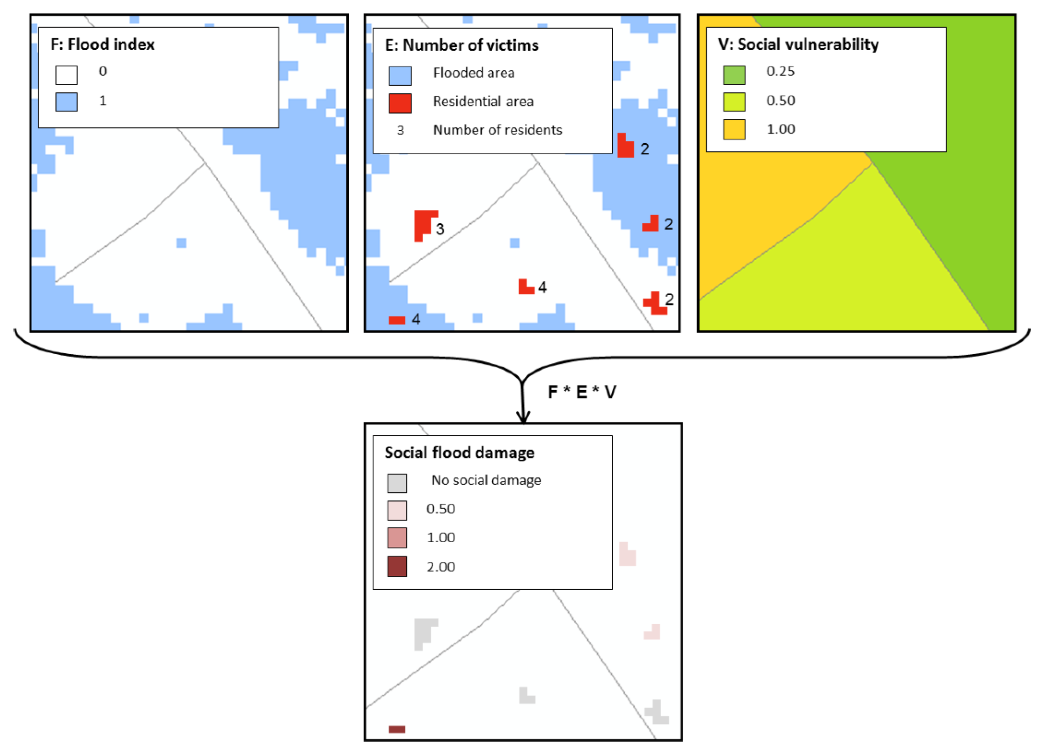
While, luckily, fatalities are often very limited, nevertheless, floods can still have huge societal impacts. In addition to the methodology to calculate the number of fatalities, the socio-human damage where there is a loss of independence of vulnerable groups was also determined. Direct socio-human damage with loss of independence of vulnerable groups due to floods is the impact of floods in which vulnerable individuals in a community lose their independence to the extent that it is life-threatening [75]. The social impact of a flood is measured by multiplying the number of persons exposed (E) with the flood index (F) and the social vulnerability index (or the maximum social damage map, V) [76].
Amongst other groups, the poorest and socially marginalized segments of the population are highly vulnerable to floods [77]. Coninx et al. (2007) tried to identify the most vulnerable population groups by integrating a so-called social vulnerability index [78]. In order to identify these groups, Coninx et al. (2007) relied on the social flood vulnerability index (SFVI) of the Flood Hazard Research Centre (FHRC), which is included in the Multi-Coloured Manual of 2013 [66]. This study identified these following vulnerable groups: people older than 75, people with health conditions, and single parents, and four parameters identifying financial deprivation: unemployment, no basic comfort (houses without a toilet, bathroom, or central heating), no car, and tenants.
A study by Van Ackere et al. (2019) translated these vulnerable group categories to the case of Flanders, Belgium (by taking all the available data into account) [76]:
- The number of beneficiaries with the right to an increased allowance;
- The number of persons with a disability;
- The number of non-Europeans and Eastern Europeans;
- The number of people older than 75;
- The number of single-parent families.
Although the indicators mentioned above broadly correspond with the indicators of the SFVI, Van Ackere et al. (2019) added nationality and house type to this list. Therefore, nationalities are grouped and classified accordingly on the basis of their vulnerability [79]. This composite index is used to estimate the number of households that face the toughest conditions and are the most vulnerable to flooding. As a consequence, an area that is not flooded will have a flood index equal to zero, thus, the social impact will also be zero.
The methodology is shown schematically in Figure 13. If the methodology is followed for flood maps of different return periods, it is also possible to measure the social risk per year.
2.3.3. Disruption Potential of a Society
The FLIAT methodology is enriched with a vulnerability assessment methodology that rates the existence of a latent probability that a society could collapse. This accounts for the fallout of vital infrastructures (e.g., a power grid, evacuation road, bridge, etc.) or functions (e.g., police station, hospital, etc.) that are necessary for the daily function of a society. For example, roads that are used to evacuate inhabitants will have a higher score of importance than roads that are less important for a community.
Vulnerable vital functions and infrastructure
To distinguish between the various types of functions and infrastructure, enterprise activity codes (NACE) were used. By expert judgement, a list of vulnerable functions was created (see Table 3). Hereby, command-centres were taken into account (e.g., police stations, fire stations, etc.), which were important to maintain and preserve functions elsewhere. Additionally, functions that were important for shelter (e.g., sport halls) or functions that were vulnerable themselves (e.g., children gardens, etc.) were considered. This list of vulnerable and vital functions and infrastructure requires special attention in terms of communication, evacuation, etc.
The advantage of using NACE codes to classify which specific vulnerable function is located in a particular building is the possibility to distinguish extensively detailed classes from each other. For example, for education, there are 35 divergent groups, among them ‘technical, vocational and special secondary education,’ ‘higher education,’ ‘sports and recreation education,’ ‘nursery education,’ ‘extraordinary primary education,’ etc. The same multi-subcategorization applies to industry, government agencies, small- and medium-sized enterprises, etc. Besides vulnerable functions, vulnerable and vital infrastructures (such as bridges, evacuation roads, etc.) were included in the FLIAT database and accounted for in the disruption potential calculation of a society.
Because the FLIAT prototype runs with PostgreSQL/PostGIS, it was easy to filter out all vital infrastructures and functions with all their important data (e.g., flood characteristics, including flood depth, flood velocity, location, construction age, etc.) with simple SQL queries.
3. Case Study
3.1. Case Study 1: Economic Impact Assessment of a Coastal Flood Scenario Along the Belgian Coast
The Belgian coastline is about 65 km long [81], consisting mostly of sandy beaches with sea walls in front of the area with a high building and population density. A large part of this sandy coastline has been subjected to erosion of the dunes for several decades. To prevent further erosion by currents and waves, groynes were built. Beach nourishments have been carried out regularly to compensate for the erosion of the coastline and to protect against storm surges [82].
In this case study, the economic damage assessment of buildings for the Belgian coast is performed for a coastal flood, using the event “in situ” of 2015 for a storm surge level (referred to the peak water level at Ostend) of +8 m TAW (Second General Levelling). The flood is simulated with the tool Mike FLOOD. The economic impact assessment is executed by the LATIS tool and the FLIAT tool for comparison. To date, damage curves for buildings only take into account the water depth in Flanders. Therefore, the economic damage calculation considers solely this flood parameter (although FLIAT can work easily with multiple flood parameters). Since the data included in the LATIS tool has, by default, a resolution of 5 m and has no NACE code linked to each building, data of footprints of buildings and the linking of the NACE codes to these footprints are established for the economic damage calculation with both the LATIS tool and the FLIAT tool.
3.1.1. LATIS Tool
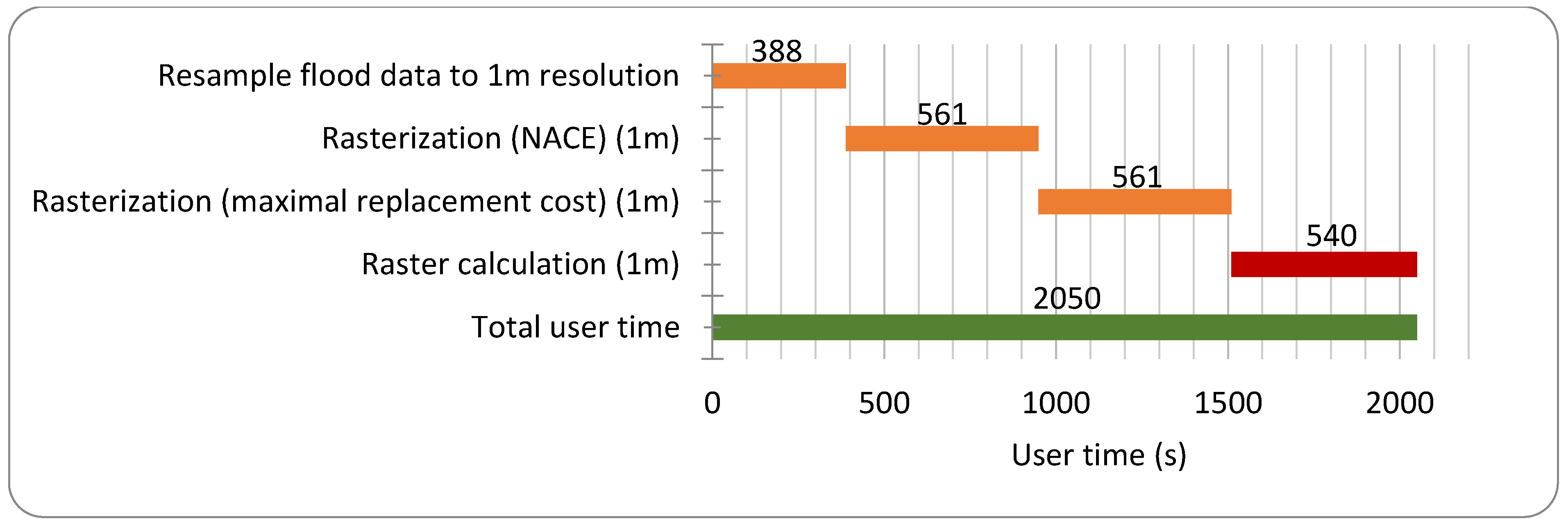
Since LATIS doesn’t come with a conversion tool to convert shape files into raster data, the ArcGIS conversion tool was used. After creating a raster file for every building with the representative maximal replacement value and the NACE code(s), the final raster calculation can be computed. This was done for a resolution of 5 m (see Figure 15) and a resolution of 1 m (see Figure 16) and was computed on a desktop with a i7-4770 3.4 GHz processor.
3.1.2. FLIAT Tool
Likewise, the calculation of economic damage due to the coastal flood event was done with the FLIAT tool. To calculate the economic damage, the raster data files of the water depth, rise velocity, and the horizontal velocity first needed to be uploaded. Because multiple server connections can be handled simultaneously, the FLIAT upload process allowed the files to stream in parallel. As a result, the time to upload all the raster files to the FLIAT server took only a few seconds for the entire Belgian coast (see Figure 17). After a quick raster calculation, the raster files were then saved into a structured PostgreSQL database. At this point, the raster data were automatically converted in parallel into multiple polygons.
When vector data of buildings was saved into the PostgreSQL database and NACE codes were linked with these buildings, the footprint polygons of the buildings could be split up into polygons, whereby every polygon had unique flood characteristics compared with their neighbouring polygons (as see in Figure 10c). Finally, the economic damage can be calculated in parallel (see Figure 17 and Figure 18c) using the Standard Method (see Equation (1)). This has been computed on a Linux server with 24 Intel(R) Xeon(R) CPU E5-2420 0 @ 1.90 GHz.
3.1.3. Statistical Analysis
The total economic damage calculated with the FLIAT tool for the Belgian coast is estimated at 4.8 billion EUR for the coastal flood event. To compare the raster approach with the FLIAT tool, the following statistical measures were used:
- Mean error (ME) indicates the degree of bias. A positive ME means that the predictions (total economic damage calculated with raster approach) are an overestimation, while a negative value signifies an underestimation of these prediction values:
- Mean absolute percentage error (MAPE):
- Root mean square error (RMSE) represents the standard deviation of the differences between predicted values and observed values:
- R² indicates how well the predicted data match the observations:with N representing the number of observations, z() as the observed values, as the predicted values, and as the mean observed value.
First, the measures of accuracy were calculated for the LATIS tool with respect to the FLIAT tool for the entire Belgian coast (see Table 4).
3.2. Case Study 2: Social Impact Assessment of a Pluvial Flood in Ghent, Belgium
Ghent is a city in the Flemish region of Belgium with an area of 156.18 square kilometres and approximately 257,000 inhabitants [83]. Ghent is a major tourist and economic midpoint in the Belgian province of East Flanders. Ghent was founded as a settlement at the confluence of the rivers Scheldt and Leie in the Late Middle Ages. The port of Ghent generated an annual direct value added of 3575.4 million EUR and a direct employment of 27602 FTE in 2016 [84]. In addition to the substantial economic input of the port for the city of Ghent, tourism also makes an enormous contribution. Lodging and food and beverage sectors constitute 8.1% of all industry in Ghent [85].
In this case study, the social damage assessment of Ghent was executed for a pluvial flood, using the event “in situ” of 2050 for heavy rainfall with a return period of 20 years, simulated by Flanders Hydraulics Research with a resolution of 5 m by 5 m. The pluvial flood event was simulated with InfoWorks ICM by the engineering firm Arcadis [81]. Because the horizontal and vertical flood speed was too low, the number of people at risk could be neglected. The loss of independence of vulnerable groups is now calculated with the LATIS and the FLIAT tool.
3.2.1. LATIS Tool
Since the pluvial flood event was simulated considering buildings and other infrastructures as obstacles (see Figure 5), flood meshes did not overlay any building footprint. Therefore, as mentioned before, it was not possible to calculate the social damage due to this specific flood event with a raster approach, even after converting the data into raster data.
3.2.2. FLIAT Tool
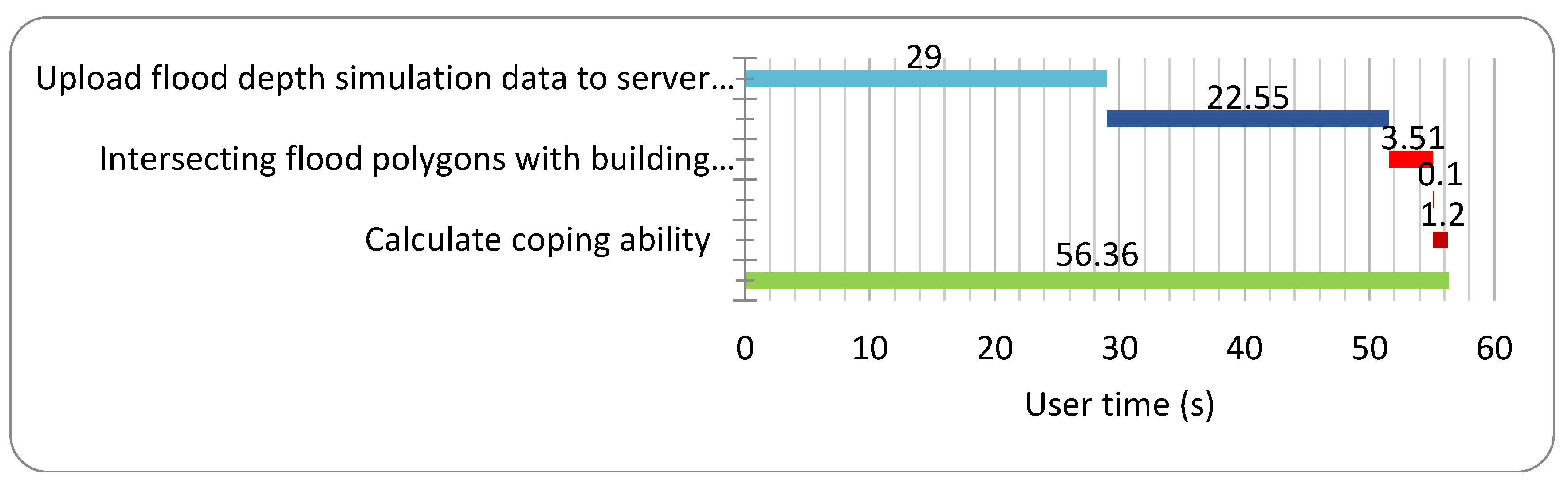
At this time, the FLIAT database was used to calculate the social damage assessment for this specific flood event. Amongst many other data, this FLIAT database contained the most up-to-date building footprints, with multiple datasets (e.g., social index [76], number of inhabitants or estimation of number of inhabitants, NACE code, average height, etc.). Because of this, it was possible to quickly calculate the loss of independence of vulnerable groups after uploading the pluvial flood simulation to the FLIAT database. The time to upload the flood data to the server had a small bottleneck in user time (with an upload speed of 67 Mbps). The loss of independence of vulnerable groups due to a pluvial flood with a return period of 20 years for the event “in situ” in 2050 for the city of Ghent was computed after 56.36 s (see Figure 19). This was computed on a Linux server with 24 Intel(R) Xeon(R) CPU E5-2420 0 @ 1.90 GHz.
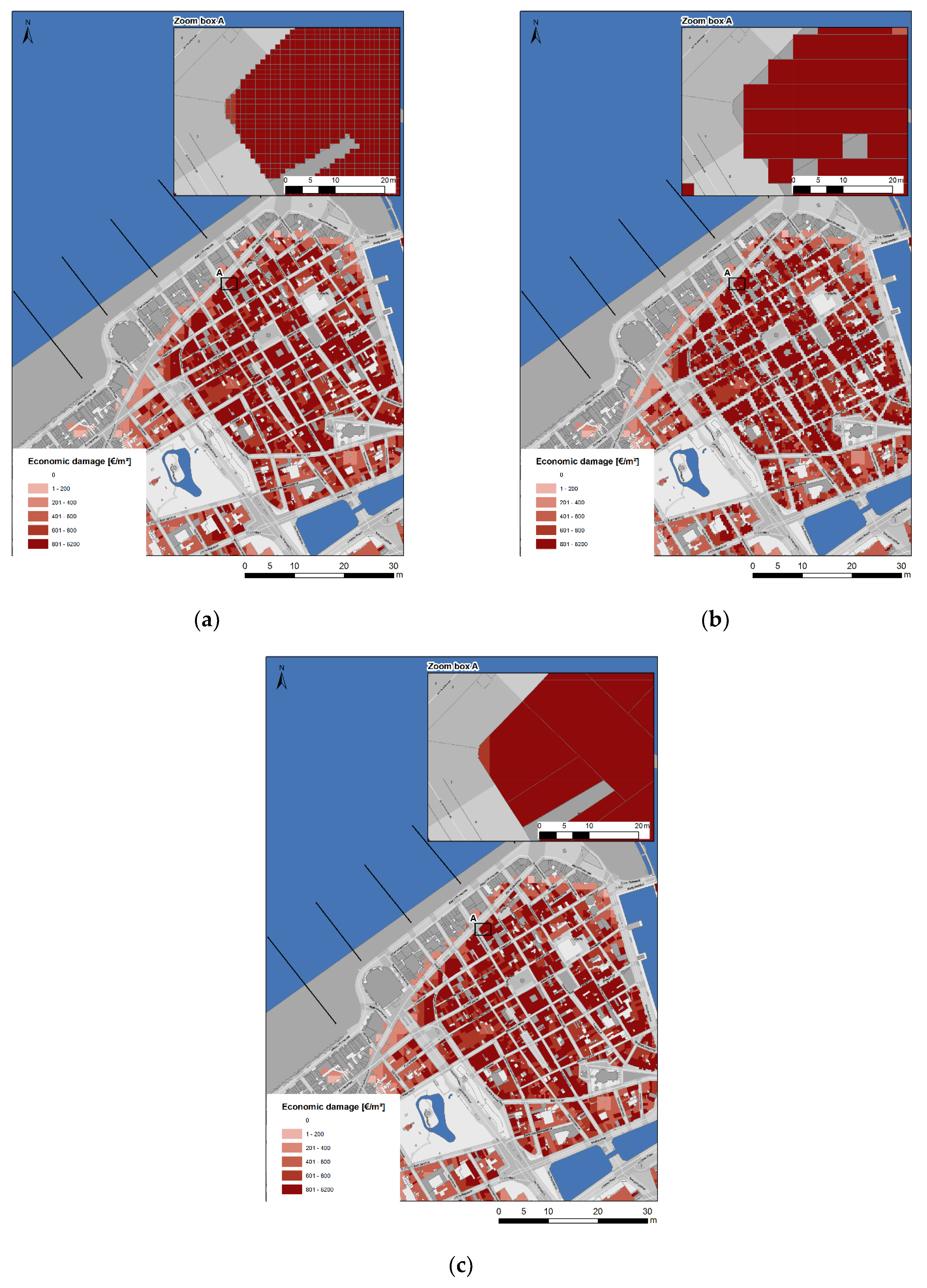
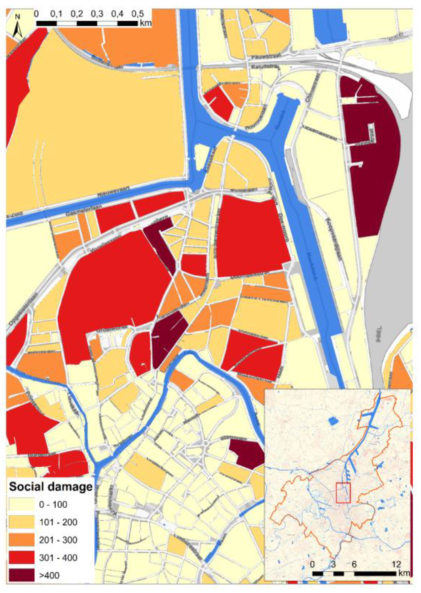
The output of the loss of independence of vulnerable groups can be seen in Figure 20.
3.3. Case study 3: Economic Impact Assessment of a Fluvial Flood in Ghent, Belgium
In this case study, an economic damage assessment resulting from pluvial floods was performed with the LATIS tool and the FLIAT tool with a return period of 1000 years for the road network of the city considering the event “in situ” in 2015. To date, damage curves for road networks only take into account the water depth in Flanders. Therefore, the economic damage calculation considered only this flood parameter. Again, to compare these two tools, the same road network with multiple subcategories was used.
3.3.1. LATIS Tool
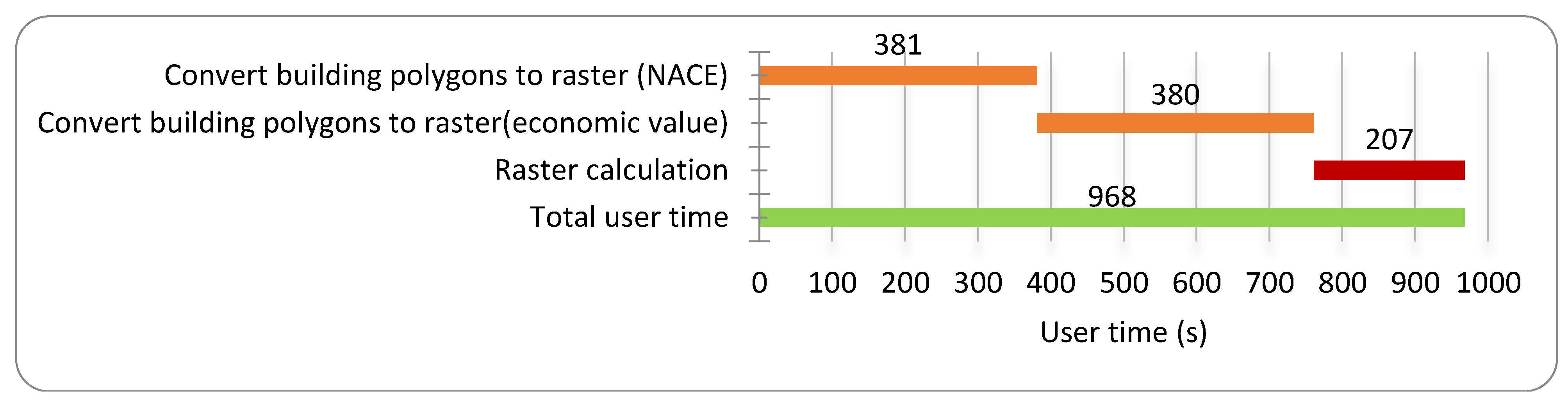
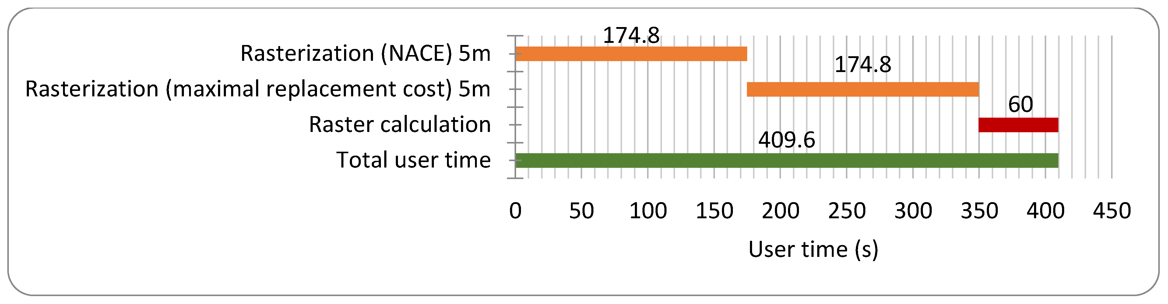
Since the pluvial flood was represented by irregular meshes, the road network, as well as the pluvial flood data, had to be converted to raster data before the economic impact of this pluvial flood can be calculated. The conversion from polygons to raster data was done by using the ArcToolbox function ‘polygon conversion to raster’. Unfortunately, the conversion of flood data must be done for the water depth and the subcategory of the road network separately (see Figure 21 and Figure 22), and it was computed on a desktop with a i7-4770 3.4 GHz processor.
3.3.2. FLIAT Tool
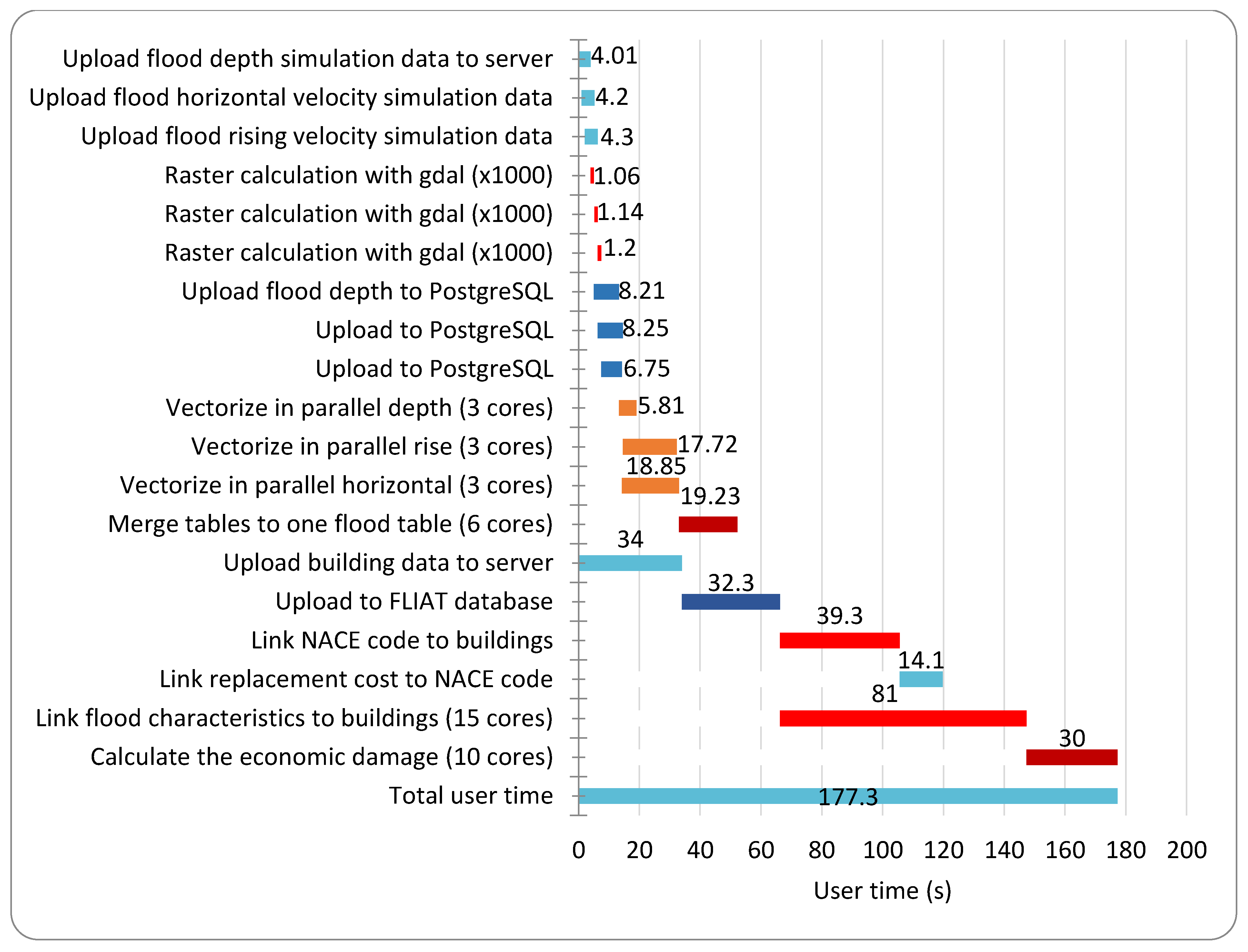
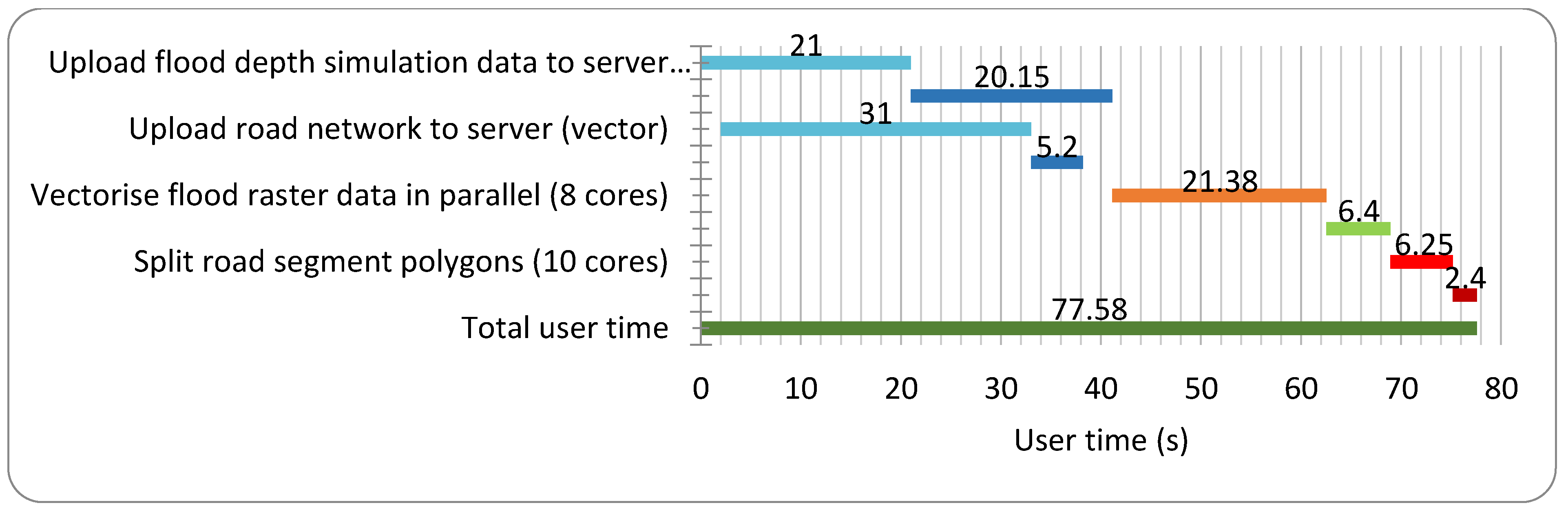
First, the fluvial flood raster data was uploaded to the server, and this was saved in the FLIAT database. Both water depth and road network data were uploaded to the server and saved to the PostgreSQL database simultaneously. The flood data was then vectorised in parallel using 8 cores, thereafter only the flooded road network segments were selected. These flooded road segment polygons were split into polygons in which every polygon had unique flood characteristics compared with their neighbouring polygons. Finally, the economic damage calculation was carried out (see Figure 23). This was computed on a Linux server with 24 Intel(R) Xeon(R) CPU E5-2420 0 @ 1.90 GHz.
The output of the FLIAT tool can be seen in Figure 24c.
3.3.3. Statistical Analysis
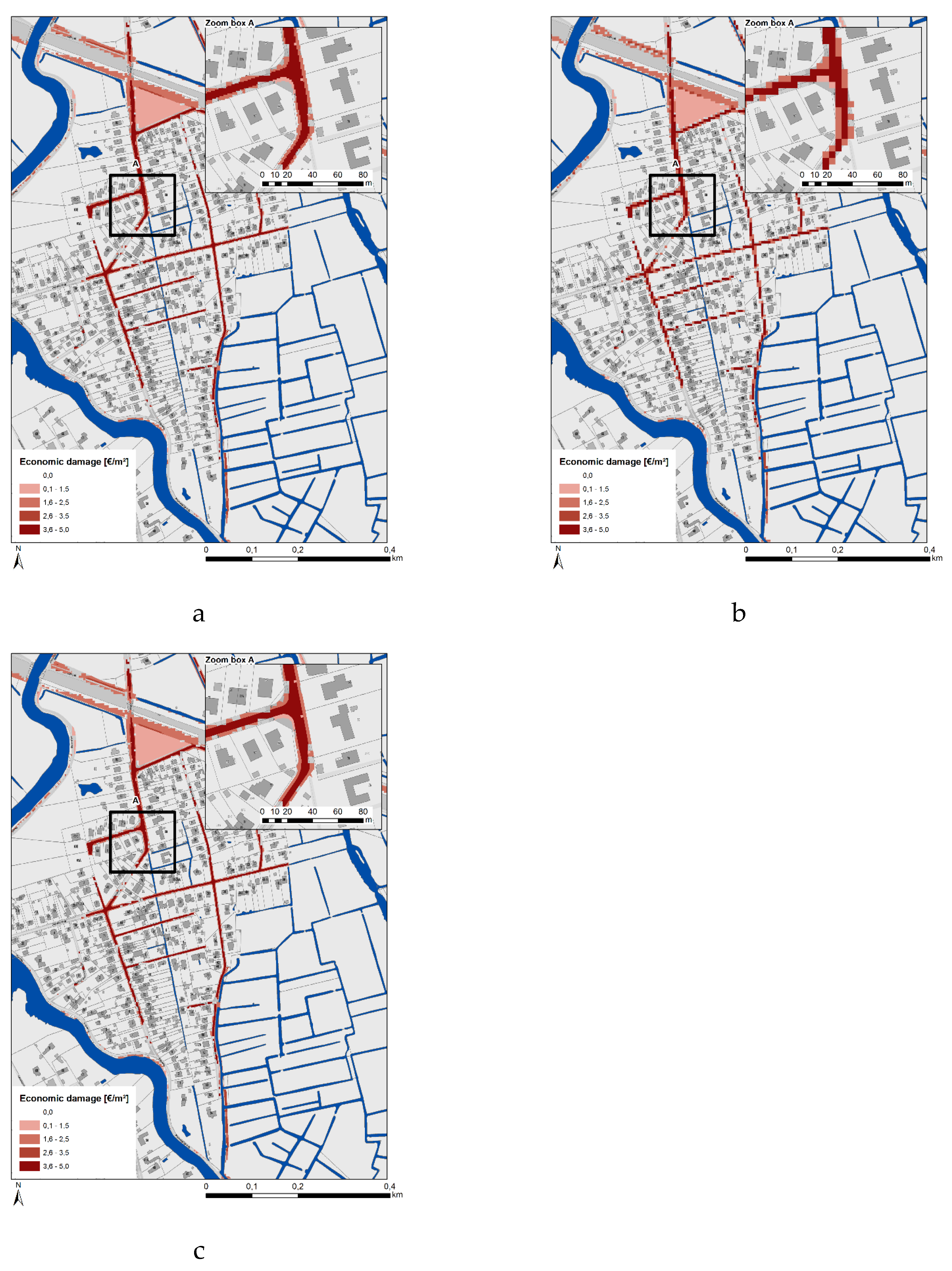
The total economic damage resulting from the pluvial flood event, calculated with the FLIAT tool for the city of Ghent, was estimated at 4 million EUR for the road network. Next, the road network was divided into multiple subcategories (e.g., motorway, bicycle path, etc.). For each of these categories, it became possible to calculate the total economic damage. First, the measures of accuracy were calculated for the LATIS tool with respect to the FLIAT tool for the whole city of Ghent (see Table 7).
4. Discussion
4.1. Accuracy of the FLIAT Tool with Respect to the LATIS Tool
To evaluate the accuracy of the LATIS and FLIAT tool, the same source land use data, demographic data, and damage curves were used. It was then possible to measure the error between raster approach and the FLIAT approach due to conversion of the source data in the LATIS tool without variations in the methodology between the two tools. The results of this study showed that the LATIS tool and the FLIAT tool calculated the same economic damage for large areas, as the errors were averaged out in the LATIS tool (see Table 4 and Table 7). When looking at a more detailed scale (e.g., per street (see Table 10) or per category (see Table 9)), a raster-based approach performed poorly, especially with a 5 m resolution.
The MAPE in Table 4 suggested that there was no significant error between the output of the FLIAT tool and the raster approach when considering the total economic damage of a large area, such as the entire Belgian coast, resulting from a coastal flood event. Nevertheless, it was clear that the FLIAT tool performed more accurately than the LATIS tool when the economic damage calculation per building block was compared, especially when the economic damage calculation in LATIS was performed with a 5 m resolution.
4.2. Comparison of Calculation Speeds of the FLIAT Tool with Respect to the LATIS Tool
LATIS was originally developed with a raster approach since a vector-based calculation was too computationally intensive without the use of parallel processing and spatial indexes. Due to the enhanced insights and the improvement in server performance and computing power, the FLIAT tool can outperform a raster-based damage assessment tool like LATIS in terms of computation time (see Figure 21, Figure 22 and Figure 23). The upload process to the PostgreSQL database experienced significant bottlenecking (see Figure 23), but since the Internet speed continues to rise, this will diminish in time.
4.3. Growth Opportunities of the FLIAT Tool
In the near future, the FLIAT tool will be able to quickly and accurately detect and use real flood characteristics in impact assessment studies of an infrastructure or other land use using doors and door thresholds, basement openings, windows, and other flood impact-influencing variables. The FLIAT tool also has the potential to take into account the stability of an infrastructure against the power of a flood event. The addition of this data will refine the damage calculation of flood events on buildings and other infrastructures. As shown in Figure 7, the FLIAT prototype does not embed the whole elaborated methodology; it is not yet possible to calculate the cultural or ecological impact resulting from floods with FLIAT, and the multi-criteria analysis must be developed. Together with the socio-economic, ecologic, and cultural impact assessment, the FLIAT methodology concludes with a priority map. This priority map provides scenarios for how a society should adapt to future climate change. As a result, the use of SQL queries to list all vital organizations and infrastructures that are crucial to preventing the disruption of a society will be available when creating a priority adaptation roadmap.
4.4. Installation and Usability of LATIS and FLIAT Tools
The LATIS tool can only be installed on a Windows platform, and the source data package must be transferred before the tool can be used. With a data set of more than 150 Gb, which will only increase when the resolution of the source data is changed to 1 m or less instead of 5 m, the installation is a cumbersome process. Additionally, updates must be done manually, so the data used is not necessarily up to date. In contrast with the LATIS tool, the FLIAT tool is cross-platform (e.g., Windows, OSX, Linux, etc.) and can run on a variety of devices (e.g., desktops, laptops, servers, and high-performing infrastructures (HPC)).
4.5. Consideration of the Entire Building
For the scenario where the flood is simulated by taking objects (e.g., buildings, infrastructures, etc.) in the landscape into account as obstacles and displaying where the flood meshes touch the building (see Figure 8), the entire building is immediately considered as affected by the flood. Unfortunately, using this method, the impact of floods for large buildings will be overestimated since the impact of the building is calculated by using the worst-case flood characteristic of one of the touching meshes. To overcome this problem, further research is needed on the behaviour and impact of floods on indoor buildings.
4.6. Usability Outside Flanders
In Flood Impact Assessment studies, data (e.g., land use data, economic data, flood simulation data, etc.) is a necessity. As soon as the necessary data is available, the FLIAT tool can also be used outside Flanders.
5. Conclusions
This paper describes the development of a flood impact assessment tool (FLIAT), which computes the socio-economic impact and the disruption potential of a society to obtain a priority map after a multi-criteria analysis. This tool works with a vector approach by using a relational database that can easily handle multiple metadata of vital infrastructures, crucial buildings, etc., which is necessary when considering the disruption potential of a society. Hereby, it is not a necessity to run the FLIAT tool with additional data or by using more detailed data compared with the current damage assessments. Nevertheless, this FLIAT tool can be used in detailed flood impact studies, for example when a (societal) cost-benefit analysis of individual measures (or a group of measures in a limited area) is made. Because FLIAT uses a vector approach, it can handle flood data in irregular meshes, as well as raster-based flood data, after converting it to vector-based flood data. The fact that FLIAT is programmed to compute with a vector approach is one of the most notable differences between FLIAT and other developed impact assessment tools (e.g., LATIS for Belgium [10], FLEMO for Germany [16], the Multi-Coloured Manual for the UK [66], HAZUS for the USA [67], and SSM-2017 for the Netherlands [14]). By using parallel computation, the FLIAT tool can immediately compute the impact of floods on a community. The FLIAT tool helps engineers, environmental agencies, and local governments accurately detect and define the priority protection zones in terms of socio-economic damage and social disruption resulting from flood events, on the basis of the uploaded flood simulation data (or occurred flood events) of a specific region. FLIAT can be used in cost-benefit analyses of, for example, sewerage and road construction projects and the construction of (coastal) protection infrastructures, and it makes the tool valuable as a decision-making tool for priority adaptation guidelines, measures, and policy recommendations. Since time is key when disasters strike urban environments, this tool can save lives and win time in the process of evacuating inhabitants and recovering a society as quickly as possible. This tool is written in Python using an open source Postgresql/PostGIS database. Consequently, the tool is accessible, as there is no need for expensive GIS software or multi-model databases (for example ArcGIS, Oracle database, etc.).
Author Contributions
S.V.A. developed the calculation methodology, developed the FLIAT tool and wrote the paper; J.B., W.V., A.D.W. and P.D.M. upgraded the text where needed.
Funding
This research is funded by the Institute of Science and Technology in Flanders (IWT Flanders) and fits into the framework of the CREST (Climate Resilient Coast) project.
Acknowledgments
The authors would like to thank the reviewers for their helpful comments and suggestions for improving this manuscript.
Conflicts of Interest
The authors declare no conflict of interest. The founding sponsors had no role in the design of the study; in the collection, analyses or interpretation of data; in the writing of the manuscript; and in the decision to publish the results.
References
- Chen, Y.; Zhou, H.; Zhang, H.; Du, G.; Zhou, J. Urban flood risk warning under rapid urbanization. Environ. Res. 2015, 139, 3–10. [Google Scholar] [CrossRef] [PubMed]
- Hartmann, T. Contesting land policies for space for rivers—Rational, viable, and clumsy floodplain management. J. Flood Risk Manag. 2011, 4, 165–175. [Google Scholar] [CrossRef]
- Tempels, B.; Hartmann, T. A co-evolving frontier between land and water: Dilemmas of flexibility versus robustness in flood risk management. Water Int. 2014, 39, 872–883. [Google Scholar] [CrossRef]
- Lebbe, L.; Van Meir, N.; Viaene, P. Potential Implications of Sea-Level Rise for Belgium. J. Coast. Res. 2008, 242, 358–366. [Google Scholar] [CrossRef]
- Silva, M.M.; Costa, J.P. Urban Floods and Climate Change Adaptation: The Potential of Public Space Design When Accommodating Natural Processes. Water 2018, 10, 180. [Google Scholar] [CrossRef]
- Mees, H.L.P.; Driessen, P.P.J.; Runhaar, H.A.C.; Stamatelos, J. Who governs climate adaptation? Getting green roofs for stormwater retention off the ground. J. Environ. Plan. Manag. 2013, 56, 802–825. [Google Scholar] [CrossRef]
- Oberndorfer, E.; Lundholm, J.; Bass, B.; Coffman, R.R.; Doshi, H.; Dunnett, N.; Gaffin, S.; Köhler, M.; Liu, K.K.Y.; Rowe, B. Green Roofs as Urban Ecosystems: Ecological Structures, Functions, and Services. Bioscience 2007, 57, 823–833. [Google Scholar] [CrossRef]
- Vanneuville, W.; Wolters, H.; Scholz, M. Flood Risks and Environmental Vulnerability; Europe’s Environment Agency: Copenhagen, Denmark, 2016. [Google Scholar]
- Schubert, J.E.; Sanders, B.F. Building treatments for urban flood inundation models and implications for predictive skill and modeling efficiency. Adv. Water Resour. 2012, 41, 49–64. [Google Scholar] [CrossRef]
- Kellens, W.; Vanneuville, W.; Verfaillie, E.; Meire, E.; Deckers, P.; De Maeyer, P. Flood Risk Management in Flanders: Past Developments and Future Challenges. Water Resour. Manag. 2013, 27, 3585–3606. [Google Scholar] [CrossRef]
- De Bruijin, K.M. Resilience and Flood Risk Management: A Systems Approach Applied to Lowland Rivers; Delft University: Delft, The Netherlands, 2005. [Google Scholar]
- Deckers, P.; Broidio, S.; Verwaest, T.; De Maeyer, P.; Mostaert, F. LATIS: Van Overstromingskaarten Naar Schadekaarten en Risicokaarten; Jaarboek De Aardrijkskunde: Antwerp, Belgium, 2013. [Google Scholar]
- Deltares Chapter 3: How to Setup a Flood Impact model—Delft-FIAT—Deltares Public Wiki. Available online: https://publicwiki.deltares.nl/display/DFIAT/Chapter+3%3A+How+to+setup+a+flood+impact+model (accessed on 24 May 2018).
- Kleist, L.; Thieken, A.H.; Köhler, P.; Müller, M.; Seifert, I.; Borst, D.; Werner, U. Estimation of the regional stock of residential buildings as a basis for a comparative risk assessment in Germany. Nat. Hazards Earth Syst. Sci. 2006, 6, 541–552. [Google Scholar] [CrossRef]
- Slager, K.; Wagenaar, D. Standaardmethode Schade aan LNC-waarden als Gevolg van Overstromingen; Ministerie van Infrastructuur en Waterstaat: Wageningen, The Netherlands, 2017. [Google Scholar]
- Kreibich, H.; Botto, A.; Merz, B.; Schröter, K. Probabilistic, Multivariable Flood Loss Modeling on the Mesoscale with BT-FLEMO. Risk Anal. 2017, 37, 774–787. [Google Scholar] [CrossRef] [PubMed]
- Seifert, I.; Kreibich, H.; Merz, B.; Thieken, A.H. Application and validation of FLEMOcs—A flood-loss estimation model for the commercial sector. Hydrol. Sci. J. 2010, 55, 1315–1324. [Google Scholar] [CrossRef]
- Chen, A.S.; Hammond, M.J.; Djordjević, S.; Butler, D. Flood damage assessment for urban growth scenarios. In Proceedings of the International Conference on Flood Resilience: Experiences in Asia and Europe, Exeter, UK, 5–7 September 2013; Volume 5. [Google Scholar]
- Chen, A.S.; Hammond, M.J.; Djordjević, S.; Butler, D.; Khan, D.M.; Veerbeek, W. From hazard to impact: Flood damage assessment tools for mega cities. Nat. Hazards 2016, 82, 857–890. [Google Scholar] [CrossRef]
- Bai, Y.; Liao, S.; Sun, J. Scale effect and methods for accuracy evaluation of attribute information loss in rasterization. J. Geogr. Sci. 2011, 21, 1089–1100. [Google Scholar] [CrossRef]
- Freeman, T.G. Calculating catchment area with divergent flow based on a regular grid. Comput. Geosci. 1991, 17, 413–422. [Google Scholar] [CrossRef]
- EDF-DRD. TELEMAC Modelling System, TELEMAC-2D, Principle Notes V.3.0; Report No. HE-43/94/052/A; EDF-DRD: Paris, France, 2001. [Google Scholar]
- DHI (Danish Hydaulic Institute). Mud Transport Module User Guide, MIKE21 MT, DHI Software; DHI Water Environ: Copenhagen, Denmark, 2002; Volume 110. [Google Scholar]
- Falconer, R.A. A mathematical model study of the flushing characteristics of a shallow tidal bay. Proc. Inst. Civil Eng. 1984, 77, 311–332. [Google Scholar] [CrossRef]
- Falconer, R.A. Water quality simulation study of a natural harbor. J. Waterw. Port Coast. Ocean Eng. 1986, 112, 15–34. [Google Scholar] [CrossRef]
- Bedri, Z.; Bruen, M.; Dowley, A.; Masterson, B. A Three-Dimensional Hydro-Environmental Model of Dublin Bay. Environ. Model. Assess. 2011, 16, 369–384. [Google Scholar] [CrossRef]
- Kashefipour, S.M.; Lin, B.; Falconer, R.A. Modelling the fate of faecal indicators in a coastal basin. Water Res. 2006, 40, 1413–1425. [Google Scholar] [CrossRef]
- Kashefipour, S.M.; Lin, B.; Harris, E.; Falconer, R.A. Hydro-environmental modelling for bathing water compliance of an estuarine basin. Water Res. 2002, 36, 1854–1868. [Google Scholar] [CrossRef]
- Schnauder, I.; Lin, B.; Bockelmann-Evans, B. Modelling faecal bacteria pathways in receiving waters. Proc. ICE Marit. Eng. 2007, 160, 143–153. [Google Scholar] [CrossRef]
- Ernst, J.; Dewals, B.J.; Detrembleur, S.; Pirotton, M.; Archambeau, P. Micro-scale flood risk analysis based on detailed 2D hydraulic modelling and high resolution geographic data. Nat. Hazards 2010, 181–209. [Google Scholar] [CrossRef]
- Luo, F.; Li, R. 3D Water Environment Simulation for North Jiangsu Offshore Sea Based on EFDC. J. Water Resour. Prot. 2009, 1, 1–57. [Google Scholar] [CrossRef]
- Walters, R.A. A model for tides and currents in the English Channel and southern North Sea. Adv. Water Resour. 1987, 10, 138–148. [Google Scholar] [CrossRef]
- Janin, J.M.; Lepeintre, F.; Péchon, P. TELEMAC-3D: A Finite Element Code to Solve 3D Free Surface Flow Problems. In Computer Modelling of Seas and Coastal Regions; Springer Netherlands: Dordrecht, The Netherlands, 1992; pp. 489–506. [Google Scholar]
- Kim, J.; Moin, P. Application of a fractional-step method to incompressible Navier-Stokes equations. J. Comput. Phys. 1985, 59, 308–323. [Google Scholar] [CrossRef]
- Cescutti, F.; Cefalo, R.; Coren, F. Application of Digital Photogrammetry from UAV Integrated by Terrestrial Laser Scanning to Disaster Management Brcko Flooding Case Study (Bosnia Herzegovina); Springer: Cham, Switzerland, 2018; pp. 245–260. [Google Scholar]
- Mason, D.C.; Trigg, M.; Garcia-Pintado, J.; Cloke, H.L.; Neal, J.C.; Bates, P.D. Improving the TanDEM-X Digital Elevation Model for flood modelling using flood extents from Synthetic Aperture Radar images. Remote Sens. Environ. 2016, 173, 15–28. [Google Scholar] [CrossRef]
- Costabile, P.; Macchione, F.; Natale, L.; Petaccia, G. Flood mapping using LIDAR DEM. Limitations of the 1-D modeling highlighted by the 2-D approach. Nat. Hazards 2015, 77, 181–204. [Google Scholar] [CrossRef]
- Bates, P.D.; De Roo, A.P.J. A simple raster-based model for flood inundation simulation. J. Hydrol. 2000, 236, 54–77. [Google Scholar] [CrossRef]
- Wechsler, S.P. Uncertainties associated with digital elevation models for hydrologic applications: A review. Hydrol. Earth Syst. Sci 2007, 11, 1481–1500. [Google Scholar] [CrossRef]
- Li, Z. A comparative study of the accuracy of digital terrain models (DTMs) based on various data models. ISPRS J. Photogramm. Remote Sens. 1994, 49, 2–11. [Google Scholar] [CrossRef]
- Li, Z. Variation of the accuracy of Digital terrain Models with sampling interval. Photogramm. Rec. 2006, 14, 113–128. [Google Scholar] [CrossRef]
- Schoorl, J.M.; Sonneveld, M.P.W.; Veldkamp, A. Three-dimensional landscape process modelling: The effect of DEM resolution. Earth Surf. Process. Landf. 2000, 25, 1025–1034. [Google Scholar] [CrossRef]
- Bolstad, P.; Stowe, T. An evaluation of DEM accuracy: Elevation, slope and aspect. Photogramm. Eng. Remote Sens. 1994, 60, 1327–1332. [Google Scholar]
- Toutin, T. Three-dimensional topographic mapping with ASTER stereo data in rugged topography. IEEE Trans. Geosci. Remote Sens. 2002, 40, 2241–2247. [Google Scholar] [CrossRef]
- Jenson, S.K. Applications of hydrologic information automatically extracted from digital elevation models. Hydrol. Process. 1991, 5, 31–44. [Google Scholar] [CrossRef]
- Claessens, L.; Heuvelink, G.B.M.; Schoorl, J.M.; Veldkamp, A. DEM resolution effects on shallow landslide hazard and soil redistribution modelling. Earth Surf. Process. Landf. 2005, 30, 461–477. [Google Scholar] [CrossRef]
- Saulnier, G.-M.; Beven, K.; Obled, C. Digital elevation analysis for distributed hydrological modeling: Reducing scale dependence in effective hydraulic conductivity values. Water Resour. Res. 1997, 33, 2097–2101. [Google Scholar] [CrossRef]
- Kuo, W.-L.; Steenhuis, T.S.; McCulloch, C.E.; Mohler, C.L.; Weinstein, D.A.; DeGloria, S.D.; Swaney, D.P. Effect of grid size on runoff and soil moisture for a variable-source-area hydrology model. Water Resour. Res. 1999, 35, 3419–3428. [Google Scholar] [CrossRef]
- Yu, D.; Lane, S.N. Urban fluvial flood modelling using a two-dimensional diffusion-wave treatment, part 1: Mesh resolution effects. Hydrol. Process. 2006, 20, 1541–1565. [Google Scholar] [CrossRef]
- Hardy, R.J.; Bates, P.D.; Anderson, M.G. The Importance of Spatial Resolution in Hydraulic Models for Floodplain Environments. J. Hydrol. 1999, 216, 124–136. [Google Scholar] [CrossRef]
- Bilskie, M.V.; Hagen, S.C. Topographic accuracy assessment of bare earth lidar-derived unstructured meshes. Adv. Water Resour. 2013, 52, 165–177. [Google Scholar] [CrossRef]
- Jamieson, S.; Lhomme, J.; Fortune, D. Innovations in irregular meshing to improve the performance of 2D finite volume flood simulation. In Proceedings of the FLOODrisk 2016—3rd European Conference on Flood Risk Management, Lyon, France, 17–21 October 2016. [Google Scholar]
- Van Ackere, S. FLIAT—FLood Impact Assessment Tool. Available online: www.fliat.be (accessed on 5 May 2018).
- Guttman, A. R-Trees: A dynamic index structure for spatial searching. In Proceedings of the 1984 ACM SIGMOD international conference on Management of data, Boston, MA, USA, 18–21 June 1984. [Google Scholar]
- Nguyen, T. Indexing PostGIS databases and spatial Query performance evaluations. Int. J. Geoinform. 2009, 5, 1–9. [Google Scholar]
- Mineter, M.J.; Dowers, S.; Gittings, B.M. Towards a HPC framework for integrated processing of geographical data: Encapsulating the complexity of parallel algorithms. Trans. GIS 2000, 4, 245–261. [Google Scholar] [CrossRef]
- Stojanovic, N.; Stojanovic, D. High–performance computing in GIS: Techniques and applications. Int. J. Reason. Intell. Syst. 2013, 5, 42–49. [Google Scholar] [CrossRef]
- PostGIS—Spatial and Geographic Objects for PostgreSQL. Available online: https://postgis.net/ (accessed on 15 June 2018).
- Boniface, Y. Psycopg2. Available online: https://github.com/yohanboniface/python-postgis (accessed on 25 July 2018).
- Statbel NACE-BEL 2008. Available online: http://statbel.fgov.be/nl/statistieken/gegevensinzameling/nomenclaturen/nacebel/ (accessed on 9 May 2017).
- Van Ackere, S.; Beullens, J.; De Wulf, A.; De Maeyer, P. Data Extraction Algorithm for Energy Performance Certificates (EPC) to Estimate the Maximum Economic Damage of Buildings for Economic Impact Assessment of Floods in Flanders, Belgium. Isprs Int. J. Geo-Inf. 2018, 7, 272. [Google Scholar] [CrossRef]
- GDAL: GDAL—Geospatial Data Abstraction Library. Available online: http://www.gdal.org/ (accessed on 12 June 2018).
- McKerns, M. Multiprocessing Python Package. Available online: https://github.com/uqfoundation/pathos (accessed on 24 March 2018).
- Warmerdam, F. GDAL Polygonize. Available online: https://github.com/LSDtopotools/LSDMappingTools/blob/master/gdal_polygonize.py (accessed on 12 June 2018).
- Bermúdez, M.; Zischg, A.P. Sensitivity of flood loss estimates to building representation and flow depth attribution methods in micro-scale flood modelling. Nat. Hazards 2018, 92, 1633–1648. [Google Scholar] [CrossRef]
- Ossa-Moreno, J.; Smith, K.M.; Mijic, A. Economic analysis of wider benefits to facilitate SuDS uptake in London, UK. Sustain. Cities Soc. 2017, 28, 411–419. [Google Scholar] [CrossRef]
- Scawthorn, C.; Flores, P.; Blais, N.; Seligson, H.; Tate, E.; Chang, S.; Mifflin, E.; Thomas, W.; Murphy, J.; Jones, C.; et al. HAZUS-MH Flood Loss Estimation Methodology. II. Damage and Loss Assessment. Nat. Hazards Rev. 2006, 7, 72–81. [Google Scholar] [CrossRef]
- Cammerer, H.; Thieken, A.H.; Lammel, J. Adaptability and transferability of flood loss functions in residential areas. Nat. Hazards Earth Syst. Sci. 2013, 13, 3063–3081. [Google Scholar] [CrossRef]
- Barredo, J.I. Normalised flood losses in Europe: 1970–2006. Nat. Hazards Earth Syst. Sci. 2009, 9, 97–104. [Google Scholar] [CrossRef]
- Egorova, R.; van Noortwijk, J.M.; Holterman, S.R. Uncertainty in flood damage estimation. Int. J. River Basin Manag. 2008, 6, 139–148. [Google Scholar] [CrossRef]
- Vanderkimpen, P.; Peeters, P.; Deckers, P. The impact of individual buildings on urban flood risk analysis. In SimHydro 2010: Hydraulic Modeling and Uncertainty; Sophia-Antipolis: Nice, France, 2010. [Google Scholar]
- Kellens, W.; Deckers, P.; Saleh, H.; Vanneuville, W.; De Maeyer, P.; Allaert, G.; De Sutter, R. A GIS tool for flood risk analysis in Flanders (Belgium). WIT Trans. Inf. Commun. Technol. 2008, 39, 21–27. [Google Scholar] [CrossRef]
- Maaskant, B.; Jonkman, S.N.; Kok, M. Analyse Slachtofferaantallen VNK-2 en Voorstellen voor Aanpassingen van Slachtofferfuncties; Ministerie van Infrastructuur en Waterstaat: Wageningen, The Netherlands, 2009. [Google Scholar]
- Jonkman, S.N. Loss of Life Estimation in Flood Risk Assessment; Theory and Applications. Ph.D. Thesis, Technical University, Delft, The Netherlands, 2007. [Google Scholar]
- Gordon, R. The Social System as Site of Disaster Impact and Resource for Recovery. Aust. J. Emerg. Manag. 2004, 19, 16–22. [Google Scholar]
- Van Ackere, S.; Beullens, J.; Broidioi, S.; De Maeyer, P. Assessment of intangible losses in flood damage calculations: Quantifying the social impact of floods in Flanders. 2018; Manuscript in preparation. [Google Scholar]
- Otto, I.M.; Reckien, D.; Reyer, C.P.O.; Marcus, R.; Le Masson, V.; Jones, L.; Norton, A.; Serdeczny, O. Social vulnerability to climate change: A review of concepts and evidence. Reg. Environ. Chang. 2017, 17, 1651–1662. [Google Scholar] [CrossRef]
- Coninx, I.; Bachus, K. Integrating Social Vulnerability to Floods in a Climate Change Context. In Proceedings of the International Conference Adaptive and Integrated Water Management Coping with Complexty Uncertainty, Basel, Switzerland, 12–15 November 2007; Volume 30. [Google Scholar]
- Verhoeven, H.; Martens, A. Arbeidsmarkt en diversiteit … over de vreemde eend in de bijt. 2000. Available online: www.werk.be (accessed on 15 April 2019).
- Gandhi, U. Automating Map Creation with Print Composer Atlas—QGIS Tutorials and Tips. Available online: https://www.qgistutorials.com/en/docs/automating_map_creation.html (accessed on 25 July 2018).
- Deronde, B.; Houthuys, R.; Debruyn, W.; Fransaer, D.; Van Lancker, V.; Henriet, J.-P. Use of Airborne Hyperspectral Data and Laserscan Data to Study Beach Morphodynamics along the Belgian Coast. J. Coast. Res. 2006, 225, 1108–1117. [Google Scholar] [CrossRef]
- Ruiz Parrado, I.; Vanneste, D.; Vanderkimpen, P.; Verwaest, T.; Mostaert, F. Update Flood Risk Coastal Plain—2015: Flood Modeling Report. Version 4.0. FHR Reports; Flanders Hydraulics Research: Antwerp, Belgium, 2016. [Google Scholar]
- Statistics Belgium. Available online: http://statbel.fgov.be/nl/statistieken/cijfers/ (accessed on 9 January 2018).
- van Gastel, G. Economic Importance of the Belgian Ports: Flemish Maritime Ports and LIÈGE Port Complex—Report 2014; National Bank of Belgium: Brussels, Belgium, 2015. [Google Scholar]
- Guidea Hotel and Catering Industry in Numbers. Available online: http://guidea.incijfers.be/ (accessed on 21 August 2016).
Figure 1.
LATIS methodology to calculate the socio-economic damage and risk [10].
Figure 1.
LATIS methodology to calculate the socio-economic damage and risk [10].

Figure 2.
Standard Method using raster calculation for the LATIS flood impact analysis in Flanders, Belgium (adapted from [12]).
Figure 2.
Standard Method using raster calculation for the LATIS flood impact analysis in Flanders, Belgium (adapted from [12]).

Figure 3.
There is a loss of information when vector data (a) is converted to raster data (b), which includes the loss of features’ shape, structure, position, attribute and so on.
Figure 3.
There is a loss of information when vector data (a) is converted to raster data (b), which includes the loss of features’ shape, structure, position, attribute and so on.

Figure 4.
Example of flood data presented as a raster (a) or as unstructured, irregular meshes (b).

Figure 5.
After converting unstructured mesh-based flood data (a) into raster-based flood data (b), there is no overlap of grid cells of the flood data with the object.
Figure 5.
After converting unstructured mesh-based flood data (a) into raster-based flood data (b), there is no overlap of grid cells of the flood data with the object.

Figure 6.
The flood impact assessment tool (FLIAT) comes with a relational database that can embed multiple detailed data sets.
Figure 6.
The flood impact assessment tool (FLIAT) comes with a relational database that can embed multiple detailed data sets.

Figure 7.
FLIAT methodology, with the indication of future development (ecological and cultural damage and risk calculation and the addition of the development of a priority adaption map methodology).
Figure 7.
FLIAT methodology, with the indication of future development (ecological and cultural damage and risk calculation and the addition of the development of a priority adaption map methodology).

Figure 8.
Unstructured mesh approach for objects in the terrain (e.g., buildings, infrastructures, etc.).
Figure 8.
Unstructured mesh approach for objects in the terrain (e.g., buildings, infrastructures, etc.).

Figure 9.
Time to run the query to detect the maximum water depth d and the maximum horizontal vh and vertical vr flood velocities for a number of buildings.
Figure 9.
Time to run the query to detect the maximum water depth d and the maximum horizontal vh and vertical vr flood velocities for a number of buildings.

Figure 10.
Example of FLIAT approach to compute the impact of floods with a vector approach in which a given road (a) has multiple categories and infrastructure elements (e.g., speed bump, intersection, emergency halting-place, traffic lights, etc.). The road is converted to the same unstructured mesh structure of the flood (b), while the last figure depicts a situation where every mesh of the unstructured mesh-based flood is split up to the lowest common denominator (c).

Figure 11.
Computation time per CPU to compute the economic impact resulting from a flood with a return period of 20 years with the FLIAT tool.
Figure 11.
Computation time per CPU to compute the economic impact resulting from a flood with a return period of 20 years with the FLIAT tool.

Figure 12.
Raster-based flood data (a) is converted to polygon-based flood data (b), where each polygon represents an area with no variation in flood characteristics.
Figure 12.
Raster-based flood data (a) is converted to polygon-based flood data (b), where each polygon represents an area with no variation in flood characteristics.

Figure 13.
Schematic representation of the calculation of the social damage during floods.

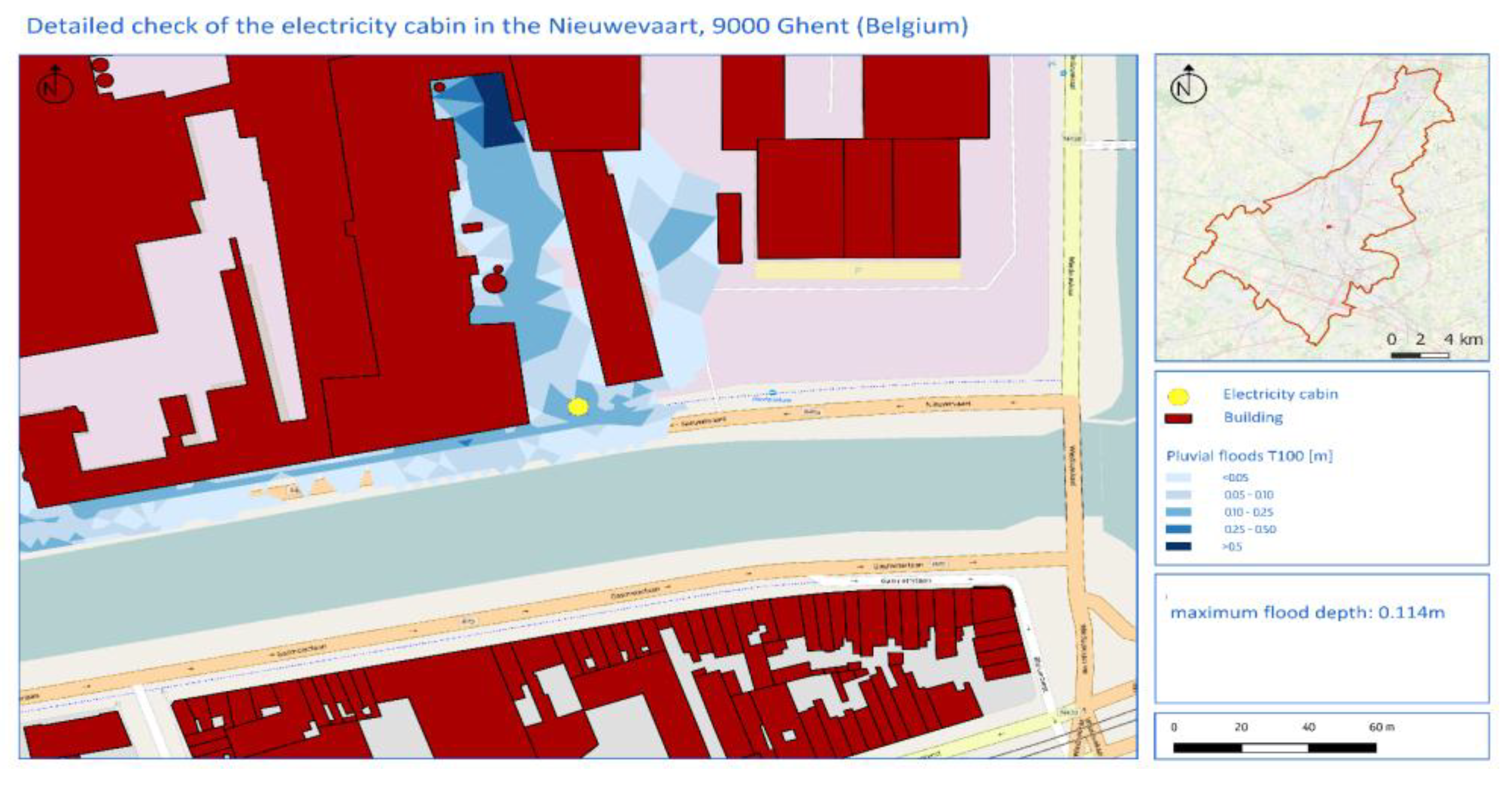
Figure 14.
Example of a detailed check map of an electricity cabin for the city of Ghent by FLIAT tool, for a pluvial flood with a return period of 100 years.
Figure 14.
Example of a detailed check map of an electricity cabin for the city of Ghent by FLIAT tool, for a pluvial flood with a return period of 100 years.

Figure 15.
User time to calculate the economic damage of a coast flood event for the Belgian coast with a resolution of 5 m.
Figure 15.
User time to calculate the economic damage of a coast flood event for the Belgian coast with a resolution of 5 m.

Figure 16.
User time to calculate the economic damage of a coast flood event for the Belgian coast with a resolution of 1 m.
Figure 16.
User time to calculate the economic damage of a coast flood event for the Belgian coast with a resolution of 1 m.

Figure 17.
User time to calculate the economic damage of a coast flood event for the Belgian coast with the FLIAT tool.
Figure 17.
User time to calculate the economic damage of a coast flood event for the Belgian coast with the FLIAT tool.

Figure 18.
Economic damage calculation with LATIS with 1 m resolution (a), 5 m resolution (b), and FLIAT (c).
Figure 18.
Economic damage calculation with LATIS with 1 m resolution (a), 5 m resolution (b), and FLIAT (c).

Figure 19.
User time to calculate the loss of independence of vulnerable groups for a road network in Ghent resulting from a fluvial flood event (return period 1000 years) with a raster approach (5 m resolution).
Figure 19.
User time to calculate the loss of independence of vulnerable groups for a road network in Ghent resulting from a fluvial flood event (return period 1000 years) with a raster approach (5 m resolution).

Figure 20.
Loss of independence of vulnerable groups resulting from pluvial floods in Ghent.

Figure 21.
User time to calculate the economic impact for a road network in Ghent resulting from a fluvial flood event (return period 1000 years) with a raster approach (5 m resolution).
Figure 21.
User time to calculate the economic impact for a road network in Ghent resulting from a fluvial flood event (return period 1000 years) with a raster approach (5 m resolution).

Figure 22.
User time to calculate the economic impact for a road network in Ghent resulting from a fluvial flood event (return period 1000 years) with a raster approach (1 m resolution).
Figure 22.
User time to calculate the economic impact for a road network in Ghent resulting from a fluvial flood event (return period 1000 years) with a raster approach (1 m resolution).

Figure 23.
User time to calculate the economic impact for a road network in Ghent resulting from a fluvial flood event (return period 1000 years) using the FLIAT tool.
Figure 23.
User time to calculate the economic impact for a road network in Ghent resulting from a fluvial flood event (return period 1000 years) using the FLIAT tool.

Figure 24.
Economic damage calculation resulting from fluvial flood with LATIS with 1 m resolution (a), 5 m resolution (b), and FLIAT (c).
Figure 24.
Economic damage calculation resulting from fluvial flood with LATIS with 1 m resolution (a), 5 m resolution (b), and FLIAT (c).


Table 1.
Example of a building saved in the PostgreSQL/PostGIS database.
| ID | Height of Building (m) | Area (m²) | Geometry | (…) |
|---|---|---|---|---|
| 408765 | 10.43 | 543 | 01060000208010(…) | (…) |
Table 2.
Examples of enterprise activity codes (NACE 2008) [60].
Table 2.
Examples of enterprise activity codes (NACE 2008) [60].
| ID | NACE | Description |
|---|---|---|
| 408765 | 47113 | retail sale in non-specialized stores where foodstuffs and stimulants predominate (sales area between 100 m² and less than 400 m²) |
| 408765 | 91020 | museum |
| 408765 | 84242 | local police station |
| 408765 | 4773001 | pharmacy |
Table 3.
List of the selected vulnerable functions with their corresponding NACE code.
| Vulnerable functions | NACE code (2008) |
|---|---|
| Police station | 84241 |
| Fire station | 84250 |
| Hospital/ emergency department | 86109 |
| City hall | 84114 |
| Rehabilitation centres and care institutions (disabled, psychiatry) | 86104, 86904, 87203, 87205, 87209 |
| Colleges and universities | 85421, 85422, 85429, 85410 |
| Nursery education | 85101, 85102, 85103, 85104, 85105, 85106, 85109 |
| Primary schools | 85201, 85202, 85203, 85204, 85205, 85206, 85209, 85311 |
| Secondary schools | 85312, 85313, 85314, 85319, 85321, 85322, 85323, 85324, 85325, 85326, 85329, |
| Service flats | 87302 |
| Railway stations, bus stations, and freight terminals | 5221001 |
| Tourist and historical sites, monuments, and tourist attractions | 91030 |
Table 4.
Measures of accuracy for the LATIS tool with respect to FLIAT tool for the whole Belgian coast (for N = 1).
Table 4.
Measures of accuracy for the LATIS tool with respect to FLIAT tool for the whole Belgian coast (for N = 1).
| ME (EUR) | MAPE (%) | RMSE (EUR) | R² | |
|---|---|---|---|---|
| Raster approach, resolution 1 m | 332908 | 0.00 | 332908 | - |
| Raster approach, resolution 5 m | −5604980 | 0.29 | 5604980 | - |
Table 5.
Statistical analysis of LATIS tool with respect to FLIAT tool for statistical sectors of the Belgian coast.
Table 5.
Statistical analysis of LATIS tool with respect to FLIAT tool for statistical sectors of the Belgian coast.
| ME (EUR) | MAPE (%) | RMSE (EUR) | R² | |
|---|---|---|---|---|
| Raster approach, resolution 1 m | 929.91 | 0.23 | 15312.72 | 0.999 |
| Raster approach, resolution 5 m | −15660.68 | 2.83 | 136240.72 | 0.999 |
Table 6.
Statistical analysis of LATIS tool with respect to FLIAT tool for building blocks of the Belgian coast.
Table 6.
Statistical analysis of LATIS tool with respect to FLIAT tool for building blocks of the Belgian coast.
| ME (EUR) | MAPE (%) | RMSE (EUR) | R² | |
|---|---|---|---|---|
| Raster approach, 1 m resolution | 2557.33 | 1.47 | 8281.60 | 0.999 |
| Raster approach, 5 m resolution | 12176.65 | 9.76 | 50687.85 | 0.997 |
Table 7.
Statistical analysis of the LATIS tool with respect to the FLIAT tool for the entire road network in Ghent (N = 1).
Table 7.
Statistical analysis of the LATIS tool with respect to the FLIAT tool for the entire road network in Ghent (N = 1).
| ME (EUR) | MAPE (%) | RMSE (EUR) | R² | |
|---|---|---|---|---|
| Raster approach, 1 m resolution | 32.00 | 0.00% | 32.00 | - |
| Raster approach, 5 m resolution | 5077.97 | 1.94% | 5077.97 | - |
Table 8.
Statistical analysis of the LATIS tool with respect to the FLIAT tool for every district road network in Ghent.
Table 8.
Statistical analysis of the LATIS tool with respect to the FLIAT tool for every district road network in Ghent.
| ME (EUR) | MAPE (%) | RMSE (EUR) | R² | |
|---|---|---|---|---|
| Raster approach, 1 m resolution | 84.83 | 0.21 | 89.70 | 0.999 |
| Raster approach, 5 m resolution | 1706.19 | 2.33 | 2415.00 | 0.999 |
Table 9.
Statistical analysis of the LATIS tool with respect to the FLIAT tool for each separate category of road network in Ghent.
Table 9.
Statistical analysis of the LATIS tool with respect to the FLIAT tool for each separate category of road network in Ghent.
| ME (EUR) | MAPE (%) | RMSE (EUR) | R² | |
|---|---|---|---|---|
| Raster approach, 1 m resolution | 20.41 | 1.93 | 28.06 | 0.999 |
| Raster approach, 5 m resolution | 461.14 | 18.92 | 813.12 | 0.999 |
Table 10.
Statistical analysis of the LATIS tool with respect to the FLIAT tool for each separate street of the road network in Ghent.
Table 10.
Statistical analysis of the LATIS tool with respect to the FLIAT tool for each separate street of the road network in Ghent.
| ME (EUR) | MAPE (%) | RMSE (EUR) | R² | |
|---|---|---|---|---|
| Raster approach, 1 m resolution | 8.36 | 1.94 | 14.05 | 0.999 |
| Raster approach, 5 m resolution | 149.16 | 23.78 | 273.47 | 0.998 |
© 2019 by the authors. Licensee MDPI, Basel, Switzerland. This article is an open access article distributed under the terms and conditions of the Creative Commons Attribution (CC BY) license (http://creativecommons.org/licenses/by/4.0/).
Share and Cite
MDPI and ACS Style
Van Ackere, S.; Beullens, J.; Vanneuville, W.; De Wulf, A.; De Maeyer, P. FLIAT, An Object-Relational GIS Tool for Flood Impact Assessment in Flanders, Belgium. Water 2019, 11, 711. https://doi.org/10.3390/w11040711
AMA Style
Van Ackere S, Beullens J, Vanneuville W, De Wulf A, De Maeyer P. FLIAT, An Object-Relational GIS Tool for Flood Impact Assessment in Flanders, Belgium. Water. 2019; 11(4):711. https://doi.org/10.3390/w11040711
Chicago/Turabian StyleVan Ackere, Samuel, Jochem Beullens, Wouter Vanneuville, Alain De Wulf, and Philippe De Maeyer. 2019. "FLIAT, An Object-Relational GIS Tool for Flood Impact Assessment in Flanders, Belgium" Water 11, no. 4: 711. https://doi.org/10.3390/w11040711
Note that from the first issue of 2016, this journal uses article numbers instead of page numbers. See further details here.