Water-Worked Gravel Bed: State-of-the-Art Review

Abstract

In a natural gravel-bed stream, the bed that has an organized roughness structure created by the streamflow is called the water-worked gravel bed (WGB). Such a bed is entirely different from that created in a laboratory by depositing and spreading gravels in the experimental flume, called the screeded gravel bed (SGB). In this paper, a review on the state-of-the-art research on WGBs is presented, highlighting the role of water-work in determining the bed topographical structures and the turbulence characteristics in the flow. In doing so, various methods used to analyze the bed topographical structures are described. Besides, the effects of the water-work on the turbulent flow characteristics, such as streamwise velocity, Reynolds and form-induced stresses, conditional turbulent events and secondary currents in WGBs are discussed. Further, the results form WGBs and SGBs are compared critically. The comparative study infers that a WGB exhibits a higher roughness than an SGB. Consequently, the former has a higher magnitude of turbulence parameters than the latter. Finally, as a future scope of research, laboratory experiments should be conducted in WGBs rather than in SGBs to have an appropriate representation of the flow field close to a natural stream.

1. Introduction

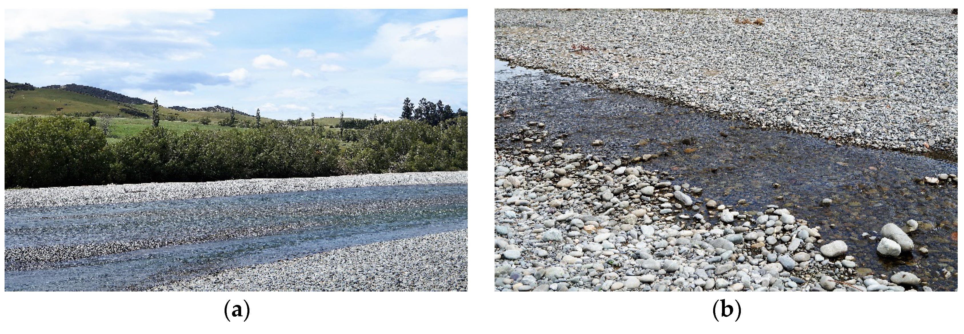
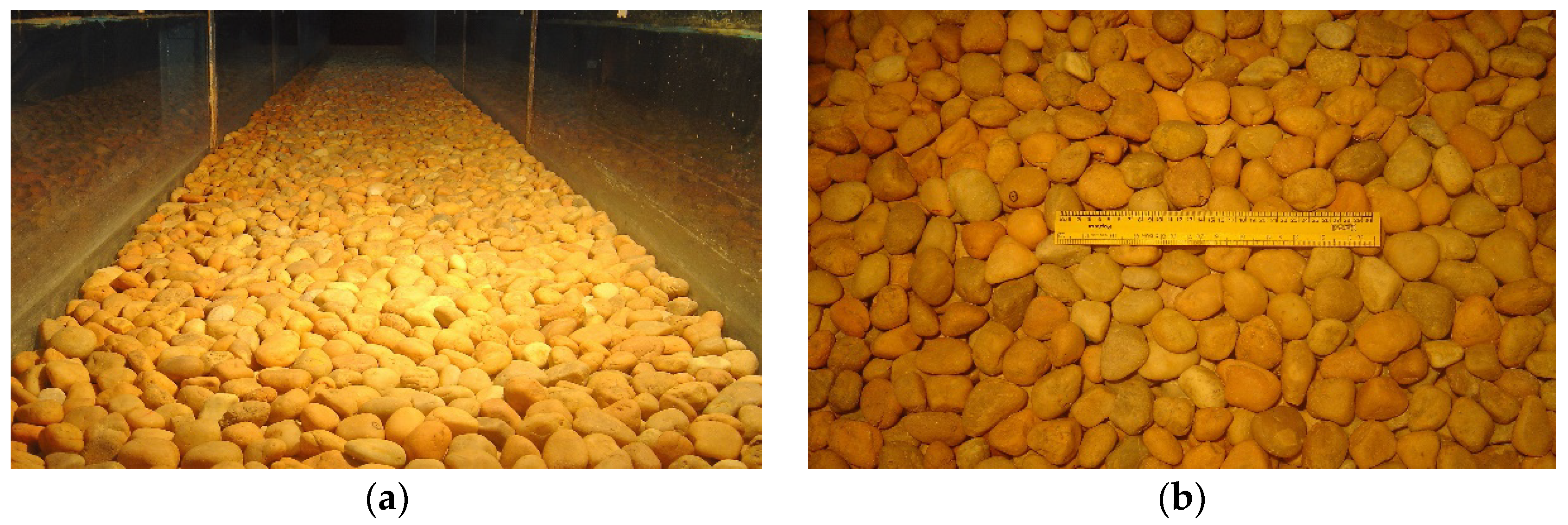
The topic of natural gravel-bed streams remains a continued research interest for several decades owing to its practical importance. The multifaceted fluid–particle interfaces yield spatial flow heterogeneities, in addition to temporal intermittencies, especially in the near-bed flow zone. It is therefore imperative to comprehend the turbulent flow physiognomies that arise from these complex turbulence mechanisms in natural streams to accurately estimate the resistance to flow and/or sediment transport rate. In fact, the bed surface topography in a natural gravel-bed stream possesses a spatially multifaceted, but coherently organized bed structure, because it is created by the natural erosion and deposition processes governed by continual flood cycles. In this process, a water-worked gravel bed (WGB) is developed in a natural gravel-bed stream (Figure 1). Specifically, water-worked refers to the work done by the flowing water on the sediment bed, for which the transport of sediments occurs in a natural stream. Hence, the gravel-bed produced by the action of flowing water is called a WGB. In contrast, in laboratory experimental studies, manmade gravel-bed is prepared by depositing and spreading gravels into the flume for a given thickness. Such a bed is called a screeded gravel bed (SGB) (Figure 2). The bed surface topography for such a bed is unorganized and randomly poised, being different from that of a WGB, even for a given identical gravel size distribution in both beds. Nonetheless, in the laboratory, a WGB can be produced if an SGB is water-worked, which can mobilize the surface gravels over a sufficiently long period until the transport of gravels ceases. To the best of the authors’ knowledge, a review on the studies done on WGBs has not yet been compiled, although there exist several compilations on the studies done on SGBs.

The aim of this article is therefore to compile a comprehensive state-of-the-art review of the most important laboratory experimental research on WGBs by analyzing the results scientifically. Attention is primarily paid to the WGB topography structures, time-averaged flow field, turbulent stresses, conditional turbulent events and secondary currents. In some cases, the results in WGBs are compared with those in SGBs.

2. Analysis of Bed Roughness Structures in WGBs

As an earlier practice, river engineers used the particle-size distribution curve to characterize the bed roughness. Bathurst [1] proposed the Nikuradse’s equivalent roughness k_s approximately to be 3–3.5 d₈₄, where d₈₄ is the 84th percentile of a particle-size distribution belonging to the range of 240–500 mm. However, the roughness height k_s cannot be estimated considering only a single gravel size, e.g., d₈₄, because other factors, such as gravel shape, orientation, alignment and structural arrangements, are of equal importance, providing significant impact on the estimation of the roughness height k_s [2,3,4,5,6,7]. Considering this fact, Kirchner et al. [5] were the first to measure the friction angle of the sediment mixtures having median size d₅₀ ranging 1.2–12 mm in both WGBs and SGBs. They observed that the difference in friction angles increases with a decrease in gravel size. Tp To quantify the impact of water-work on the bed roughness structures, they compared the difference between the bed roughness structures in WGBs that were created by the water action and SGBs that were manmade. The results reveal that, for an identical particle-size distribution, the distributions of friction angles in a WGB and an SGB are different, because the friction angles in the former are smaller than those in the latter. They argued that the difference in the friction angles occurs owing to the difference in gravel packing geometries in these beds. Hence, they concluded that the friction angle measured in an SGB cannot be directly applicable to a WGB.

2.1. Use of Probability Density Function

Skewness and kurtosis coefficients are deemed to be important properties, as they provide useful information about the distributions of roughness structures. Kirchner et al. [5], Nikora et al. [8], Marion et al. [9] and Aberle and Nikora [10] performed preliminary analysis of the roughness structures in WGBs and SGBs. They found that the probability distribution functions (PDFs) of roughness structures in both beds follow the normal distribution, but possess skewness values of opposite signs. The PDFs in WGBs are positively skewed, while they are negatively skewed in SGBs. Marion et al. [9] analyzed the PDFs of roughness structures at different time intervals during the creation of a WGB by the sediment transport process. The PDFs of roughness structures were narrow at the initial periods, but, as time elapsed, they became flatter having increased skewness. Although in their study the PDFs of different roughness structures were unable to identify the particle scale features uniquely, the WGB PDFs are positively skewed and the SGB PDFs are negatively skewed. Aberle et al. [10] also had similar observations. They postulated that, in a WGB, the roughness structure is composed of course gravels with finer particles filling the interstices of gravels. This causes the reduction of the surface elevation of the roughness structure with respect to the mean bed level. As a result, the PDF is positively skewed. Buffin-Bélanger et al. [11] also reported similar results. Later et al. [12] performed experiments in WGBs and an SGB. In their study, the WGBs were created by feeding sediment at the upstream end of the flume. Besides, to understand the impact of feeding rate on the roughness structures, they generated three WGBs at three different feeding rates. These WGBs, namely Fed bed 1, Fed bed 2 and Fed bed 3, were created at feeding rates of 0.0624 kg m⁻¹, 0.0922 kg m⁻¹ and 0.152 kg m⁻¹, respectively. The PDFs of these four beds revealed that the SGB has a slightly negatively skewed distribution of the roughness structure, while the WGBs have a very slightly positively skewed distribution (Figure 3). Moreover, they found that, with an increase in feeding rate, the skewness value decreases. Interestingly, in both the WGBs and the SGB, the kurtosis coefficients were found to be positive, indicating a leptokurtic curve.

2.2. Use of the Second-Order Structure Function

Although the PDFs of the roughness structures provide information about the bed surface features and the difference between a WGB and an SGB, they do not provide any information about the degree of organization of the surface particles. For an immobile gravel-bed with a Gaussian distribution of roughness structure, a quantitative evaluation of roughness structure can be done by using a second-order structure function. Nikora et al. [8] were the pioneers of applying the second-order structure function to ascertain the behavioral features in a WGB. They argued that, if a roughness structure is treated as a random field, then the roughness description can be reduced to two-dimensional spectrum, correlation function and structure function, by using the hypothesis of local spatial homogeneity. The advantage of using the second-order structure function is that it can consider all the important parameters that influence the roughness structure. The second-order structure function is expressed as follows:

$$D(l_x,l_y)=\frac{1}{(N-n)(M-m)}{\displaystyle \sum _{j=1}^{N-n}{\displaystyle \sum _{k=1}^{M-m}{[\left|z^{\prime }(x_j+n\delta x,y_k+m\delta y)-z^{\prime }(x_j,y_k)\right|]}^2}},$$

(1)

where D(l_x, l_y) is the second-order structure function of the bed elevation, z′ is the bed surface fluctuation with respect to the mean bed elevation $\overline{z}$, l_x is the sampling interval in streamwise direction (= nδx), l_y is the sampling interval in spanwise direction (= mδy), j = 1, 2, 3, …, n, n is the number of points in streamwise direction, k = 1, 2, 3, …, m, m is the number of points in spanwise direction, and δx and δy are the sampling intervals in x and y directions, respectively. However, following the concept of Monin et al. [13], Nikora et al. [8] obtained the D(l_x, l_y) as follows:

$$D(l_x,l_y)=2({\sigma }_z^2-R(l_x,l_y)),$$

(2)

where

$$\begin{gathered} {\sigma }_z=\sqrt{\frac{1}{NM-1}{\displaystyle \sum _{i=1}^{NM}{z^{\prime }}_i^2}}\mathrm{and} \\ R(l_x,l_y)=\frac{1}{(N-n)(M-m)}{\displaystyle \sum _{j=1}^{N-n}{\displaystyle \sum _{k=1}^{M-m}[z^{\prime }(x_j+n\delta x,y_k+m\delta y)z^{\prime }(x_j,y_k)]}}. \end{gathered}$$

(3)

In Equation (3), σ_z is the standard deviation and R(l_x, l_y) is the correlation function of the bed elevations. Interestingly, Nikora et al. [8], instead of computing D(l_x, l_y) for all the measured points, computed the D(l_x, l_y = 0) and D(l_x = 0, l_y) assuming that the main anisotropy axes of the roughness coincide with their chosen x and y axes in a WGB and an SGB. From the analysis, they found that the data form both beds collapsed onto two curves, indicating the existence of two different universal classes of gravel-bed roughness.

Further, Nikora et al. [8] observed that the D(l_x, l_y) is composed of three regions: scaling, transition and saturation regions. However, the first and last regions play the main role. For a small spatial lag, the D(l_x, l_y) acts as a power function (that is, the scaling region), while, for a large spatial lag, the D(l_x, l_y) becomes constant (that is, the saturation region). Goring et al. [14] extended the work of Nikora et al. [8] by computing the second-order structure function for a two-dimensional roughness structure and obtained similar results. Later, Butler et al. [15] analyzed the roughness structure in a WGB using the fractal analysis in both streamwise and spanwise directions. To do so, they applied a two-dimensional fractal method to high-resolution digital elevation models. They identified a mixed fractal behavior with two characteristic fractal bands; one associated with the subgrain scale and the other associated with the grain scale. The subgrain and grain scales features are isotropic and anisotropic, respectively. They also observed that, owing to the streamwise orientation of the longest axis of particles, the fractal dimensions are higher in the streamwise direction than in the other directions. It implies that the effects of water-work are to modify the organization of roughness structure by increasing the surface irregularities and hence the roughness height. Then, similar to Goring et al. [14], Marion et al. [9] used Equation (2) to analyze the variation of roughness structure with time in a WGB under a mobile bed condition. They showed that the roughness structures captured at different time intervals are directly associated with the bed mobility conditions. Moreover, their second-order structure function for roughness structure depicted the development of two different grain scale classes. One grain class was developed under a static armoring condition, where the gravels formed a bed surface with strong streamwise and spanwise coherences. The other one was developed under the dynamic armoring condition, where the gravels formed a bed surface very quickly, but only with very strong streamwise coherence. However, they were unable to establish a relation between the grain scale features with the bed mobility condition. Following the method proposed by Nikora et al. [8], Cooper and Tait [12] used the second-order structure functions for roughness structures of three fed WGBs and an SGB. They calculated the correlation lengths in the WGBs and an SGB. They indicated that the correlation lengths in both streamwise and spanwise directions in the WGBs are larger than those in the SGB, confirming that the WGBs have larger scale bed features than the SGB. Later, Qin and Ng [16] performed the second-order structure function analysis in a WGB and an SGB. They found similar results as obtained by the aforementioned researchers.

2.3. Use of Higher-Order Structure Function

Owing to gravel imbrications (overlapping of gravels) and orientations, it is not always feasible to obtain a PDF of Gaussian distribution. Hence, for such a case, to quantify the features of the roughness structures in a WGB, the higher-order structure function is deemed to be an effective tool [8,10,17]. Further, the use of higher-order structure function provides multiscaling behavioral features of the roughness structure [18,19]. It is represented as follows:

$$D_p(l_x,l_y)=\frac{1}{(N-n)(M-m)}{\displaystyle \sum _{j=1}^{N-n}{\displaystyle \sum _{k=1}^{M-m}{[\left|z^{\prime }(x_j+n\delta x,y_k+m\delta y)-z^{\prime }(x_j,y_k)\right|]}^p}}$$

(4)

where D_p(l_x, l_y) is the higher-order structure function and p is the order of the moment of the structure function.

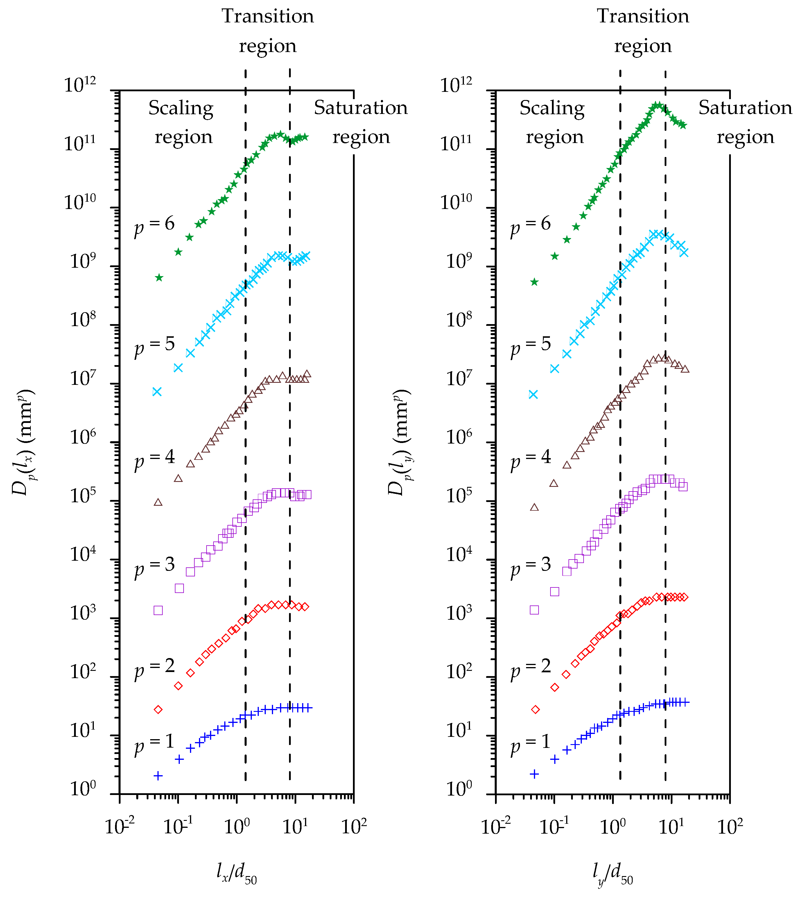
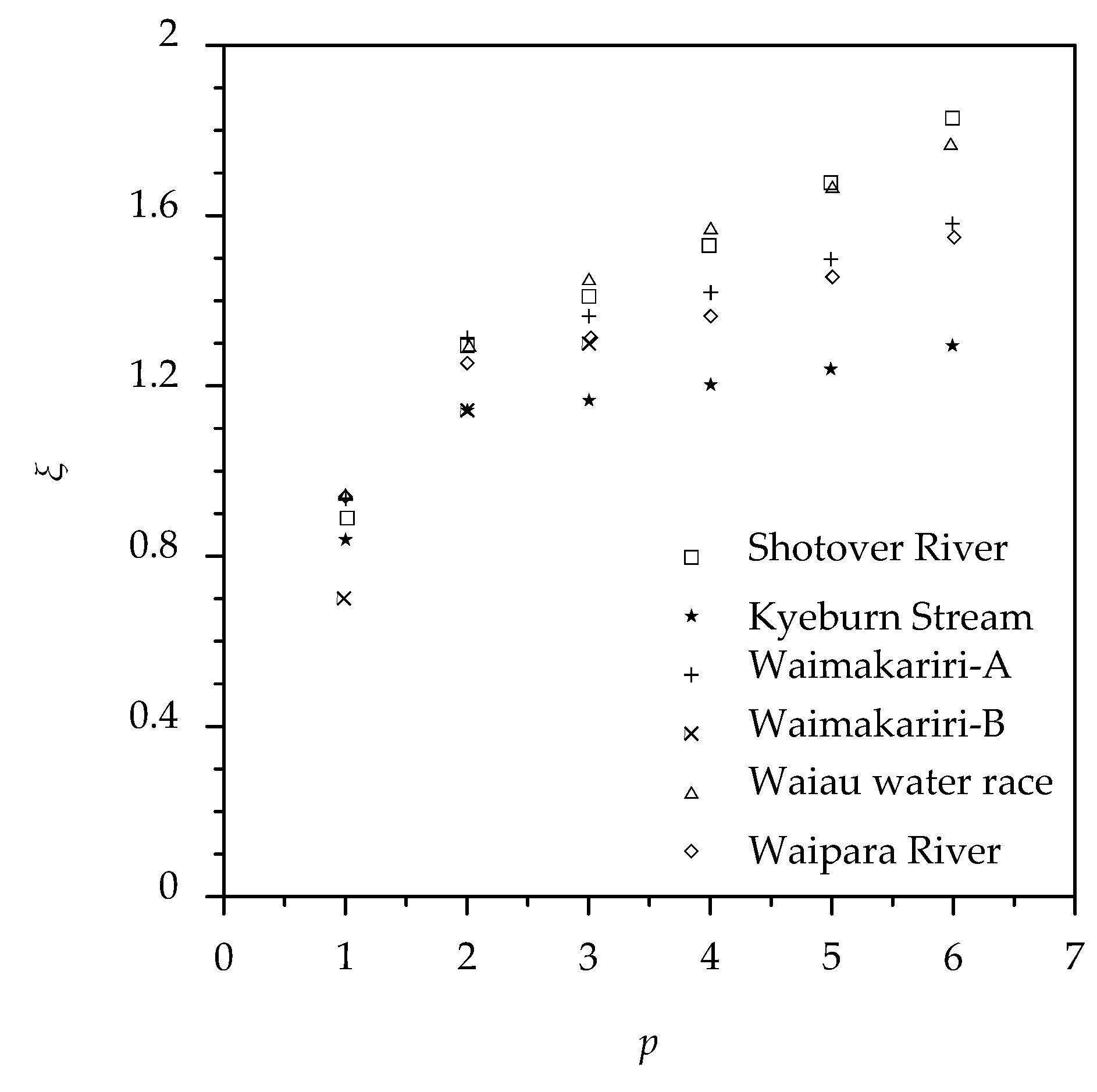
Nikora et al. [17] computed the structure function up to the sixth-order (p = 6) using the concept of Kolmogorov [20]. Similar to the second-order structure function, the shape of the D_p(l_x, l_y) can be divided into three regions: scaling, transition and saturation regions (Figure 4) [17]. Interestingly, they revealed that, in WGBs, the boundary between the scaling and transition regions is of the order of the median gravel size d₅₀, while the boundary between the transition and saturation regions is of order of d₉₀, where d₉₀ is the 90th percentile of a particle-size distribution. Akin to Nikora et al. [8], in Nikora and Walsh [17], the analysis of D_p(l_x, l_y) suggested that the grain scales are isotropic, indicating that the D_p(l_x, l_y) is independent of the axis rotation. However, within the transition region, the D_p(l_x, l_y) becomes anisotropic. Further, within the scaling region, the scaling exponent ξ plays an important role. For small values of l_x and l_y, the ξ varies linearly with p. Nevertheless, as p increases, the ξ varies nonlinearly with p, suggesting a multiscaling behavior of roughness structures in WGBs, being sensitive to the flow direction (Figure 5). The reason is attributed to the shape and the spatial arrangements of gravels [17].

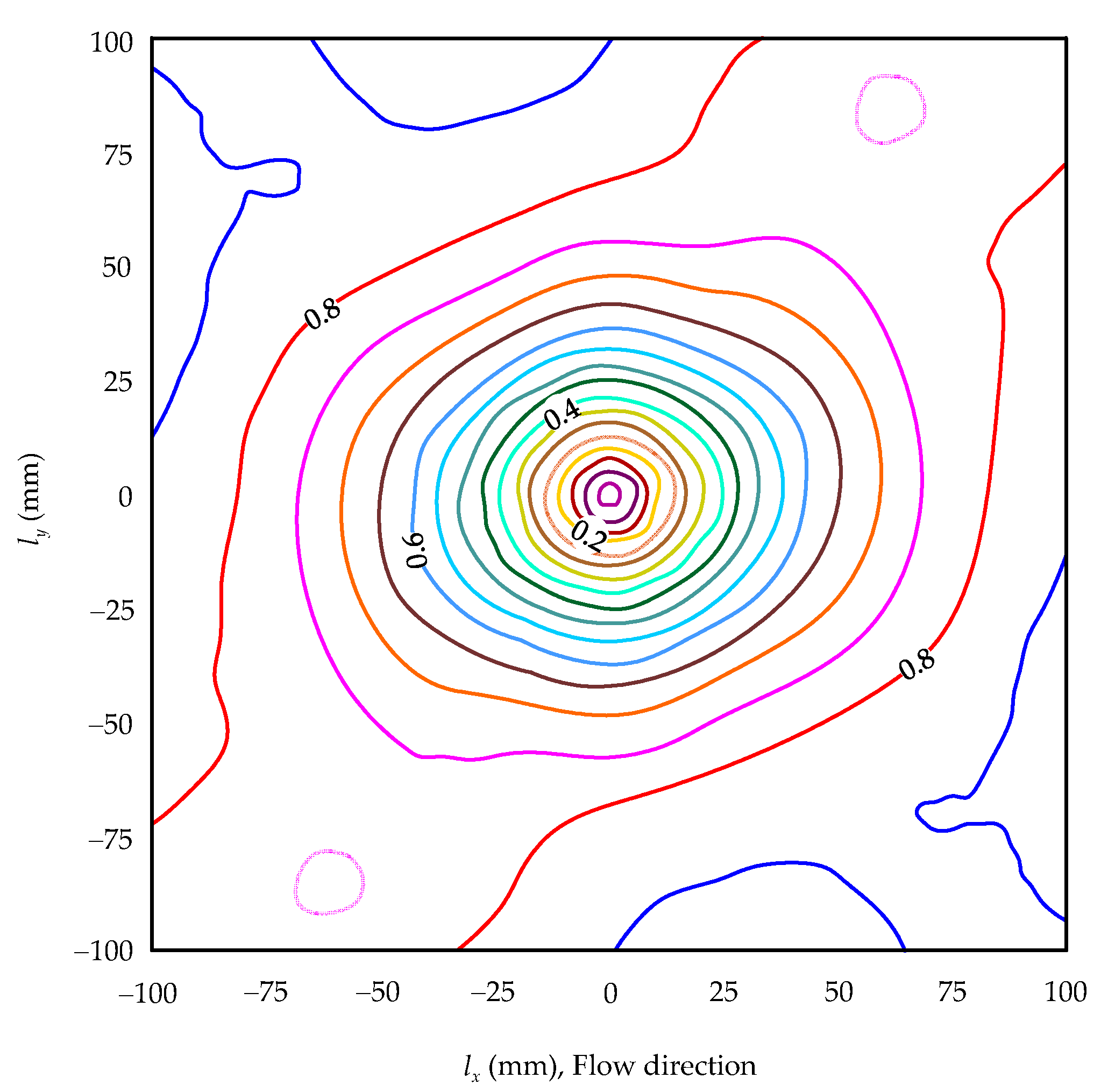
In a WGB, to understand the effects of multiscaling behavior of roughness structures in the flow direction, Aberle et al. [10] used both the second- and higher-order structure functions. They plotted the second-order structure functions in the form of contours for different armoring discharge conditions. In all cases, the contours form an elliptical shape. Similar observations were also made by Butler et al. [15] and Nikora et al. [17]. An examination of the contours reveals that, at small spatial lags in both streamwise and vertical directions, the longest axes of the nearly elliptical contours are aligned in the streamwise direction (Figure 6). It implies that the majority of gravels are to be rested on the bed keeping their longest axis in the streamwise direction [10]. They further argued that at the end of the armoring process, the gravels keep their longest axis in the streamwise direction before coming to the resting position, which is in conformity with the observations of Allen [21]. On the other hand, large gravels, which were not moved by the flow, are oriented without any directional preference. As a result, the alignment of the large contours does not match with the flow direction (Figure 6). By analyzing the higher-order structure functions in WGBs for different armoring discharge conditions (0.012–0.025 m³ s⁻¹), Aberle and Nikora [10] found that the WGB roughness structures possess multiscaling behavioral features, which is in conformity with the findings of Nikora et al. [17].

Moreover, Aberle et al. [10] stated that, although the second-order structure function shows the orientation toward the flow, it does not provide any information about the flow direction; for instance, whether it took place from right to left or left to right. Hence, they used the method proposed by Smart et al. [22] to predict the flow direction based on the gravel orientation. By using the local bed inclination at small spatial lags, the average positive and negative bed slopes can be estimated as follows:

For a positive slope [z′(x_j + nδx) − z′(x_j) > 0],

$$E_p(l_x)=\frac{1}{n_p}{\displaystyle \sum _{j=1}^{n_p}\left[\frac{z^{\prime }(x_j+n\delta x)-z^{\prime }(x_j)}{n\delta x}\right]}$$

(5)

and for a negative slope [z′(x_j + nδx) − z′(x_j) < 0],

$$E_n(l_x)=\frac{1}{n_n}{\displaystyle \sum _{j=1}^{n_n}\left[\frac{z^{\prime }(x_j+n\delta x)-z^{\prime }(x_j)}{n\delta x}\right]},$$

(6)

where E_p and E_n are the positive and negative bed slopes, respectively, and n_p and n_n are the number of positive and negative slopes, respectively.

Using Equations (5) and (6), they calculated the E_p and E_n in the WGBs and found that, at small lags, the frequency of negative slope is less than that of positive slope, owing to the gravel imbrication. Further, they revealed that the ξ of the gravels is directly associated with the armoring discharge and the individual large gravels create less complex roughness structure than a large number of small gravels.

Moreover, to determine the self-affine property and complexity of roughness structure in a WGB, estimation of the Hurst coefficient is required [8,10,12,14]. In fact, the Hurst coefficient is related to the fractal dimension. For lower values of Hurst coefficient, the fractal dimension becomes higher, and the number of significant modes that enter the evaluation of the distributed field of roughness structure also remain higher. Within the scaling region, if the Hurst coefficients in streamwise and spanwise directions are the same, then the roughness structures are isotropic within the scaling region and vice versa. Nikora et al. [8] and Cooper et al. [12] estimated the Hurst coefficients in WGBs and SGBs. They found that the Hurst coefficients in WGBs are higher than those in SGBs, indicating the roughness structures in WGBs are more complex than those in SGBs [23]. Aberle et al. [10] estimated the Hurst coefficients for armoring discharge conditions, finding that the Hurst coefficient increases with an increase in discharge and is highly dependent on the shape and orientation of gravels.

3. Turbulence Characteristics in WGBs

Flow over a gravel-bed is spatially heterogeneous and this affects the entire turbulence structure in the flow. The continuous fluid–particle interaction causes a more complex near-bed flow field, making difficult to estimate the sediment transport, the resistance to flow and important turbulence parameters in the flow. It implies that the bed topography is the primary cause to have such a complex flow field. Thus far, several studies show that the bed topography in a WGB is fairly different from that in an SGB, as mentioned in the preceding section, suggesting that the impacts of both the beds on the turbulence characteristics are different. Considering this, several researchers analyzed the effects of the WGB roughness structures on the turbulence parameters for various flow conditions.

3.1. Effects of Water-Work on Streamwise Velocity

Barison et al. [24] analyzed the time-averaged flow field over a WGB and found that the flow field is drastically affected by the roughness structure owing to the action of water-work. However, in their study, they did not analyze the bed topography precisely. Later, Buffin-Bélanger et al. [11] analyzed the spatial heterogeneity in the flow parameters, especially at the near-bed flow zone, considering three different Reynolds numbers (1.7 × 10⁵, 2.2 × 10⁵ and 2.9 × 10⁵) in a WGB. They observed that the spatial heterogeneity of the time-averaged velocity decreases with a decrease in the vertical distance, but it increases with an increase in Reynolds number. At a high Reynolds number, the spatial heterogeneity was found to be maximum in the near-bed flow zone. Further, they analyzed the mean and skewness maps of the time-averaged streamwise velocity on the horizontal plane at two different vertical distances: one near the bed and the other in the main flow layer. They observed that the mean and skewness maps for the near-bed case were more complex than those for the main flow layer case. The skewness values suggested that the shapes of the velocity distributions are different for these cases. In the near-bed flow zone, the skewness is mostly positive, while in the main flow layer, the skewness is almost negative. Buffin-Bélanger et al. [11] argued that the positive skewness values in the near-bed flow zone possibly reflect incursions of high-speed fluid streaks, while the negative values in the main flow layer indicate the incursions of low-speed fluid streaks. To be explicit, the low-speed and high-speed fluid streaks refer to the ejections and sweeps.

To understand the effects of the bed roughness structure on the spatial organization of the flow structure, Cooper et al. [25] conducted experiments on two WGBs, where the bed structure was created using unimodal and bimodal gravel mixtures. They analyzed the streamwise velocities in both the beds and found that, although the bed roughness structures are different, the spatial organization of streamwise velocities in both the beds are almost the same. Further, Cooper et al. [25] also studied the effects of relative submergence (1.2–1.9 for unimodal gravel-bed and 1.3–2 for bimodal gravel-bed) on the spatial pattern of streamwise velocity showing them in the form of contour plots. They found that, with an increase in relative submergence, the number of high-speed fluid streaks decreases, but the number of low-speed fluid streaks increases. It implies that, as relative submergence increases, the streamwise velocity distribution becomes spatially homogeneous, which is in conformity with the observations of Legleiter et al. [26]. In both unimodal and bimodal gravel-beds, they also found that, for a given slope and bed shear stress, the relative submergence provides a more significant impact on the spatial distribution of the streamwise velocity than the bed topography. Later, Hardy et al. [27] performed a time series analysis to visualize the instantaneous velocity field through a series of consecutive images in WGBs, for three different Reynolds numbers (1.3 × 10⁵, 2.5 × 10⁵ and 2.7 × 10⁵). They observed that, for all Reynolds numbers, the flows are highly inconsistent in the near-bed flow zone. Further, the turbulent structures that originate from the near-bed zone are to intrude into the main flow layer. These structures change their form and magnitude at higher Reynolds numbers, becoming more distinct, having a clearer velocity signature and a steeper upstream-dipping slope.

Thereafter, Koll et al. [28] studied the near-bed turbulent flow field over two WGBs. They kept the statistical distribution of the surface gravels identical in both the beds, but with different gravel orientations. In the first phase, they created a WGB and took the flow measurements over it. Subsequently, they rotated the surface gravels in a WGB by 90° and measured the flow field in the newly created WGB. Analysis of the double averaged (DA) streamwise velocity 〈ū〉 profiles in both the beds showed that a higher flow retardation occurs in the WGB with rotated gravels than in the original WGB. They identified that the difference in magnitude of 〈ū〉 is mainly caused by the change in near-bed turbulence rather than by the spatial distribution of time-averaged velocity.

Besides, after Nezu et al. [29], the bed topography can be considered as one of the most influencing factors in estimating the turbulence parameters. Therefore, to quantify the impact of the bed topography on the flow velocity, Pu et al. [30] carried out experiments over three different beds (a smooth bed, a WGB and an SGB), using an Acoustic Doppler Velocimeter (ADV), and compared the results. They used the following equations of log-wake laws for velocity profiles:

For smooth flow,

$$\frac{u}{u_{*}}=\frac{1}{\kappa }\ln \left(\frac{u_{*}z}{\nu }\right)+\underset{B_r}{\underbrace{\frac{1}{\kappa }\ln \left(\frac{u_{*}{z}_0}{\nu }\right)}}+\frac{2\Pi }{\kappa }{\sin }^2\left(\frac{\pi }{2}\frac{z}{h}\right),$$

(7)

and for rough (SGB and WGB) flows,

$$\frac{u}{u_{*}}=\frac{1}{\kappa }\ln \left(\frac{z+\Delta z}{k_s}\right)+\underset{B_r}{\underbrace{\frac{1}{\kappa }\ln \left(\frac{z_0}{k_s}\right)}}+\frac{2\Pi }{\kappa }{\sin }^2\left(\frac{\pi }{2}\frac{z}{h}\right),$$

(8)

where u_* is the frictional velocity, z is the vertical distance, ν is the kinematic viscosity, B_r is the constant of integration, κ is the von Kármán coefficient, Π is the Coles’ wake parameter, Δz is the virtual bed level (≈0.25 k_s, according to Dey et al. [31]), z₀ is the zero velocity level, k_s is the average roughness height, and h is the flow depth.

Pu et al. [30] used the velocity data of each bed to obtain the fitted curves for the log-wake laws (Figure 7). Interestingly, the values of B_r are lower in both the smooth and the rough (WGB and SGB) beds than the traditional values: B_r = 5.5 and 8.5 for the smooth and rough beds, respectively. Further, even though the flow conditions of both the WGB and SGB were identical, they observed that the B_r in the WGB was smaller than that in the SGB. It implies that, in the near-bed flow zone, a WGB roughness structure affects B_r and, in turn, the velocity profile. In addition, the comparison of Π values in the WGB and SGB revealed that the values of Π remain the same in the velocity profiles of both the beds, suggesting that the water-work has an insignificant impact on the Π, which mainly governs the velocity profile in the outer layer.

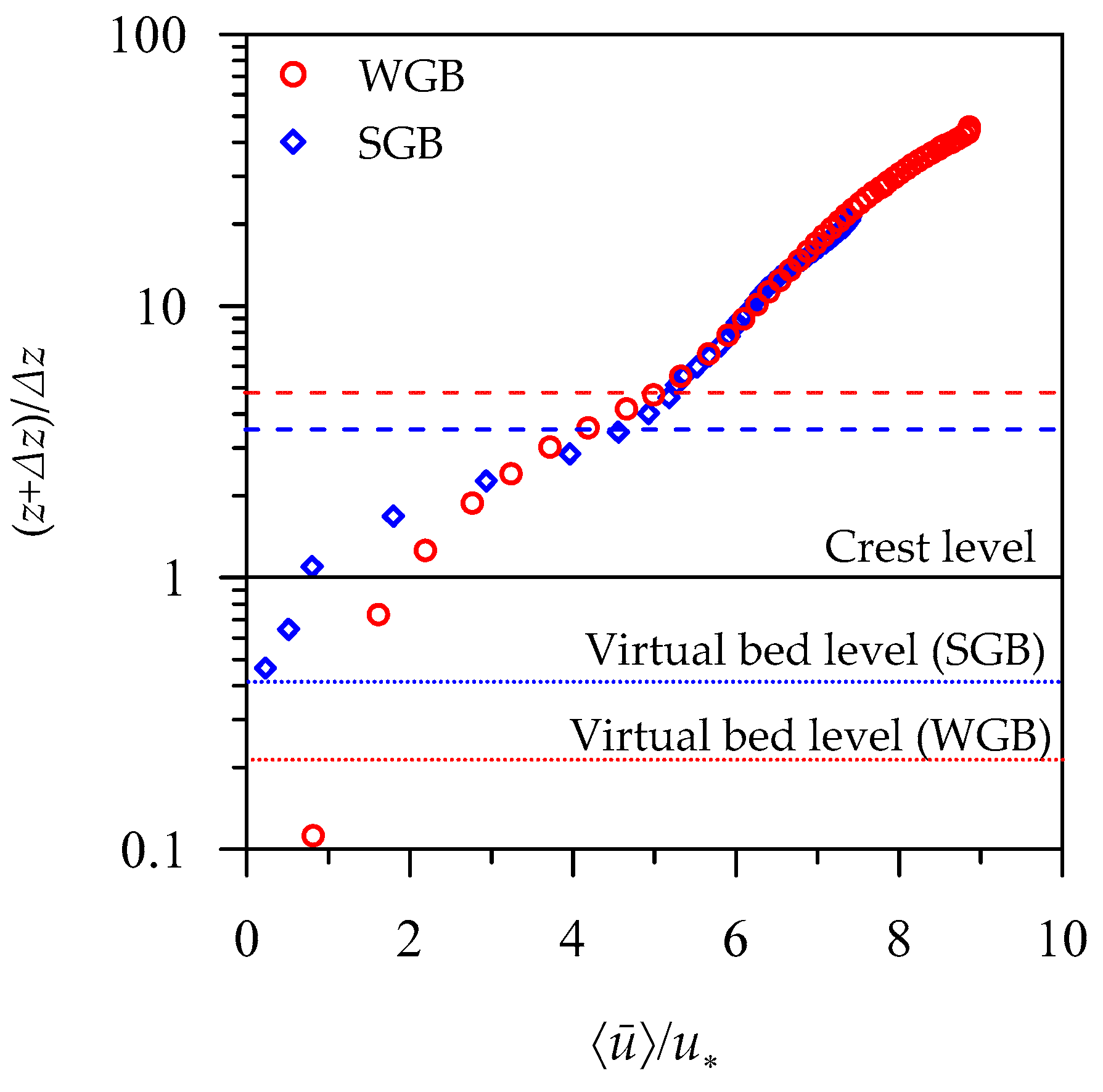
To ascertain the impact of the water-work on streamwise velocity more precisely, using a unimodal sediment mixture, Padhi et al. [32] measured streamwise velocity in a WGB using a Particle Image Velocimetry (PIV) system and compared it with that in an SGB (Figure 8). In their study, owing to the water action, the WGB roughness structure was observed to be better organized than the SGB roughness structure, where gravels were randomly sorted. Akin to other rough-flow, in the study by Padhi et al. [32], owing to the presence of gravels, the values of 〈ū〉 in both the WGB and SGB are small in the near-bed flow zone. However, they gradually increase with an increase in vertical distance, reaching a maximum at the free surface. Moreover, Padhi et al. [32] found that, close to the bed, the 〈ū〉 in the WGB is higher than that in the SGB, although the flow conditions in both the beds were alike. They argued that the well-organized roughness structure in a WGB makes the near-bed flow more streamlined than that in an SGB, inducing the 〈ū〉 to attain a higher magnitude in the former than in the latter. However, the difference in magnitudes of 〈ū〉 between a WGB and an SGB gradually diminishes, as the vertical distance increases.

3.2. Effects of Water-Work on Reynolds Shear Stresses and Form-Induced Shear Stresses

For steady, uniform flow over a macro-rough bed, the spatially averaged (SA) total fluid shear stress 〈$\overline{\tau }$〉 can be expressed as follows:

$$\langle \overline{\tau }\rangle =\langle {\tau }_f\rangle +\langle {\overline{\tau }}_{uw}\rangle +\langle {\overline{\tau }}_v\rangle ,$$

(9)

where 〈τ_f〉 is the SA form-induced shear stress (= −ρ〈$\tilde{u}\tilde{w}$〉), ρ is the mass density of fluid, ũ and $\tilde{w}$ are the spatial velocity fluctuations in the streamwise and vertical directions, respectively, 〈${\overline{\tau }}_{uw}$〉 is the SA Reynolds shear stress (= −ρ〈$\overline{u^{\prime }{w}^{\prime }}$〉), u′ and w′ are the temporal velocity fluctuations in the streamwise and vertical directions, respectively, and 〈${\overline{\tau }}_v$〉 is the SA viscous shear stress (= −ρνd〈ū〉/dz).

Although the 〈${\overline{\tau }}_{uw}$〉 remains the prevailing stress in a turbulent flow across the flow depth, the 〈τ_f〉 is the governing stress near the gravel-bed [33]. Aberle et al. [34] focused on the 〈τ_f〉 profile influenced by the roughness elements. They analyzed the spatial flow heterogeneity in terms of the 〈τ_f〉 in WGBs for different discharges. Their results infer that the magnitude of 〈τ_f〉 is small away from the crest. However, the 〈τ_f〉 increases as one moves toward the crest in the downward direction. It indicates that the ũ and $\tilde{w}$ near the bed are higher than those away from the bed, resulting in a higher magnitude of 〈τ_f〉. Further, they found that the 〈τ_f〉 profiles are similar for different discharges. Interestingly, the similarity in 〈τ_f〉 profiles is not preserved for different bed slopes. It suggests that for a given bed slope, the 〈τ_f〉 profile is independent of discharge.

Then, to study the effects of different sediment mixtures on both the 〈${\overline{\tau }}_{uw}$〉 and 〈τ_f〉, Cooper and Tait [35] analyzed all the terms of Equation (9) in two WGBs created by the unimodal and bimodal sediment mixtures. For the unimodal sediment mixture, the relative submergences varied within the range of 1.2–1.9, while, for bimodal sediment mixture, they varied within 1.3–2. They analyzed the results in terms of forces caused by the shear stresses. In doing so, they considered the fluid force caused by the 〈${\overline{\tau }}_{uw}$〉 at a given vertical distance as 〈${\overline{\tau }}_{uw}$〉ϕA₀, where ϕ is the roughness geometric function (= A_f/A₀, where A_f is the area of fluid in the averaging domain at a given elevation within the total area A₀). Above the roughness crest, ϕ = 1. Similarly, the fluid force caused by the 〈τ_f〉 at given vertical distance was obtained as 〈τ_f〉ϕA₀. They further argued that in addition to these two forces, there exists an additional force called the form drag 〈τ_d〉, which can be computed as ${\displaystyle \underset{z}{\overset{z_c}{\int }}0.5C_d\rho {\langle \overline{u}\rangle }^2{A}_e\mathrm{d}z}$, where C_d is the drag coefficient and A_e is the exposed frontal area of the grain to the fluid. However, in the analysis, they neglected the force caused by the 〈${\overline{\tau }}_v$〉 term considering that it has minimal impact on the turbulent flow. It is pertinent to mention that their analysis mainly focused on the zone below the roughness crest. Analyzing the forces, they inferred that within this zone, the vertical variations of the forces contributed from 〈${\overline{\tau }}_{uw}$〉, 〈τ_f〉 and 〈τ_d〉 with ϕ are similar and thus controlled by the geometry of the roughness elements. Moreover, they observed that with a decrease in vertical distance, the reduction in the force caused by a damping of 〈${\overline{\tau }}_{uw}$〉 is compensated by the addition of the force caused by 〈τ_d〉. Furthermore, their results showed that as the relative submergence increases, the forces contributed from the 〈${\overline{\tau }}_{uw}$〉, 〈τ_f〉, and 〈τ_d〉 increase. It suggests that for a given bed surface topography, the mechanism of momentum transfer between the fluid and particle fairly changes with an increase in relative submergence. When the results of unimodal and bimodal WGBs were compared, they found that for a given vertical distance and relative submergence, the force contributed from the 〈${\overline{\tau }}_{uw}$〉 and 〈τ_d〉 in the unimodal WGB is less than that in the bimodal WGB in the upper portion of the roughness layer and vice versa. Interestingly, in the lower portion of the roughness layers of both beds, the force caused by the 〈τ_f〉 was observed to have different vertical distributions. It indicates that for a given relative submergence, the mechanism of momentum transfer differs owing to the difference in roughness structure.

Later, Cooper et al. [36] used the experimental data of Aberle et al. [34] to quantify the spatial flow variance and the 〈τ_f〉 for different flow submergence conditions and for gravel-beds with different roughness structures. They observed that the spatial flow variance within the roughness layer is typically 4–5 times higher than that above the roughness layer. In fact, it becomes invariant to the vertical distance at a distance twice the roughness height above the crest. Owing to the increase in relative submergence, the spatial flow variance with respect to 〈τ_f〉 decreases within and above the roughness layer. However, the flow submergence does not have a significant impact on the spatial flow variance with respect to 〈${\overline{\tau }}_{uw}$〉. Further, their study infers that for different bed surface topographies, the spatial flow variance and the 〈τ_f〉 profiles vary, suggesting that the bed geometry possesses a strong control on the spatial flow variance profiles and the vertical organization of the time-averaged flow within the roughness layer.

Pu et al. [30] compared the 〈${\overline{\tau }}_{uw}$〉 profiles in a smooth bed with those in the WGB and SGB. They showed that the 〈${\overline{\tau }}_{uw}$〉 profile in the smooth bed converges with the gravity line at a shorter vertical distance than those in the WGB and SGB. Between these two rough beds, the 〈${\overline{\tau }}_{uw}$〉 profile in the WGB takes longer vertical distance to collapse on the gravity line than that in the SGB. They argued that as the WGB possesses higher roughness among all the beds, it causes the flow to have the thickest unsettled turbulence mixing layer in the near-bed flow zone, although the effects of roughness do not persist in the main flow layer. Further, regarding the magnitude of 〈${\overline{\tau }}_{uw}$〉 profile, they showed that the 〈${\overline{\tau }}_{uw}$〉 profile in a smooth bed attains the highest magnitude among all, but no explanation was given for that. Moreover, although they showed the effects of roughness on the 〈${\overline{\tau }}_{uw}$〉, the impact of roughness on the 〈τ_f〉 were not taken into consideration.

Recently, Padhi et al. [32] examined the effects of roughness on the 〈${\overline{\tau }}_{uw}$〉 and 〈τ_f〉 profiles in a WGB and an SGB. Akin to Pu et al. [30], Padhi et al. [32] found that the roughness height in the WGB was also higher than that in the SGB. However, the results of Padhi et al. [32] do not correspond to those of Pu et al. [30]. In the study by Padhi et al. [32], the 〈${\overline{\tau }}_{uw}$〉 profile in the WGB is higher than that in the SGB owing to a higher roughness height in the former than in the latter (Figure 9). They stated that a higher roughness in the WGB than in the SGB enhances the u′ and w′ values, causing an increased magnitude of 〈${\overline{\tau }}_{uw}$〉 in the WGB. The results are in agreement with those reported in Nezu and Nakagawa [29], Nikora et al. [33], Mignot et al. [37] and Dey and Das [38]. Moreover, the 〈${\overline{\tau }}_{uw}$〉 profile in the WGB collapses on the gravity line at a shorter distance than that in the SGB. It implies that, although the WGB exhibits a higher roughness height than the SGB, owing to the well-organized roughness structure in the WGB, intense flow mixing is restricted to a shorter vertical distance. Further, the 〈τ_f〉 profiles in the WGB and SGB showed that a higher roughness in the WGB than in the SGB produces large values of ũ and $\tilde{w}$ causing an increased magnitude of 〈τ_f〉 in the former than that in the latter (Figure 9). This suggests that in the near-bed flow zone, the flow is more heterogeneous in the WGB than in the SGB.

3.3. Effects of Water-Work on Reynolds Normal Stresses and Form-Induced Normal Stresses

For a heterogeneous turbulent flow, the SA streamwise and vertical Reynolds normal stresses are expressed as 〈σ_uu〉 = ρ〈$\overline{u^{\prime }{u}^{\prime }}$〉, and 〈σ_ww〉 = ρ〈$\overline{w^{\prime }{w}^{\prime }}$〉, respectively. Similarly, the streamwise and vertical form-induced normal stresses are 〈σ_fuu〉 = ρ〈$\tilde{u}\tilde{u}$〉 and 〈σ_fww〉 = ρ〈$\tilde{w}\tilde{w}$〉, respectively.

According to Aberle et al. [34], the effects of the spatial heterogeneity in bed roughness on the streamwise time-averaged velocity can be ascertained by analyzing the 〈σ_fuu〉 (Figure 10). They observed that, akin to the 〈τ_f〉 profile, the 〈σ_fuu〉 profile is small away from the crest and gradually increases, as one moves downward toward the crest. Interestingly, they found that for a given bed slope and bed roughness structure, the 〈σ_fuu〉 profiles are almost identical for all the discharges. It implies that the shape of the 〈σ_fuu〉 profiles are independent of discharge. Further, they compared the 〈σ_fuu〉 profiles obtained for different roughness structures, but for a constant bed slope. They argued that the shapes of all the 〈σ_fuu〉 profiles are similar, although their absolute magnitudes are different. This suggests that the magnitude of 〈σ_fuu〉 profiles is governed by the roughness structure. Then, they analyzed the 〈σ_fuu〉 profiles for different bed slopes, keeping the roughness structure identical. The comparison of 〈σ_fuu〉 profiles revealed that the variation of bed slope (S₀ = 0.001 to 0.01) has a significant impact on the shape of the 〈σ_fuu〉 profiles.

The spatial velocity fluctuations ũ and $\tilde{w}$ are highly affected by the relative submergence [34]. Hence, to understand the behavioral features of the ũ with respect to the relative submergence, Koll et al. [28] studied the 〈σ_fuu〉 profiles over the original and rotated WGBs. They tested two relative submergences for each bed type: for the original WGB, the relative submergences were taken as 4.4 and 3.2, while, for the rotated WGB, they were 4.5 and 3.3. They noticed that, in the near-bed flow zone, the 〈σ_fuu〉 profile increases with an increase in relative submergence. However, away from the bed, the effects of relative submergence diminish. Cooper et al. [36] examined the impact of the relative submergence on both the 〈σ_fuu〉 and 〈σ_fww〉 profiles in a WGB. In fact, they carried out the analysis for form-induced intensities, 〈σ_fuu〉^0.5 and 〈σ_fww〉^0.5. They showed that the SA streamwise form-induced intensity 〈σ_fuu〉^0.5 profiles exhibit similar shape for all the values of relative submergences. The spatial flow variance is maximum at the middle of the interfacial sublayer, gradually diminishing away from the crest and continuing up to a vertical distance equaling twice the roughness height above the crest. Further, they observed that between the crest and the vertical distance of twice the roughness height above the crest, the spatial variance is half of its peak value in all the 〈σ_fuu〉^0.5 profiles, irrespective of the bed roughness. Analysis of the impact of relative submergence on the 〈σ_fuu〉^0.5 profiles revealed that, for a given vertical distance, the magnitude of 〈σ_fuu〉^0.5 profile is inversely proportional to the relative submergence. Thus, it confirms that the relative submergence governs the 〈σ_fuu〉^0.5 profile. By contrast, the results of SA vertical form-induced intensity 〈σ_fww〉^0.5 profiles inferred that although the shapes of 〈σ_fww〉^0.5 profiles are similar to those of 〈σ_fuu〉^0.5 profiles, there is an insignificant difference in the magnitudes of 〈σ_fuu〉^0.5 profiles owing to the difference in relative submergences. Additionally, they analyzed the 〈σ_uu〉^0.5 and 〈σ_ww〉^0.5 profiles for different relative submergences. Akin to 〈σ_fuu〉^0.5 profiles, the magnitudes of 〈σ_uu〉^0.5 profiles reduce with an increase in relative submergence, confirming that these profiles are also affected by the relative submergence. Further, they found that the spatial variance in 〈σ_uu〉^0.5 profiles is approximately half of the spatial variance in the time-averaged streamwise velocity profiles. Moreover, a small variation in 〈σ_ww〉^0.5 profiles was observed owing to the change in relative submergence. It is important to mention that the spatial variance in 〈σ_ww〉^0.5 profiles is approximately half of the spatial variance in 〈σ_uu〉^0.5 profiles and equals the spatial variance in time-averaged vertical velocity profiles. This implies that the spatial flow variance in the streamwise direction is higher than that in the vertical direction.

Considering three types of beds (smooth bed, WGB and SGB), Pu et al. [30] measured the turbulence intensities in streamwise, spanwise and vertical directions. As traditionally found, the turbulence intensities are higher in the rough beds (WGB and SGB) than in the smooth bed. Further, their observations revealed that between the WGB and SGB, the WGB possesses a less even bed roughness structure than that in the SGB. It causes to have larger turbulence intensities and velocity fluctuations in the former than in the latter. It indicates that the WGB can modify the flow turbulence intensity distribution and in turn, the Reynolds normal stresses with respect to the SGB.

Recently, Padhi et al. [32] examined the 〈σ_uu〉, 〈σ_ww〉, 〈σ_fuu〉 and 〈σ_fww〉 profiles in a WGB and an SGB. Their analysis showed that owing to the higher WGB roughness height, both u′ and w′ enhance, resulting in higher values of 〈σ_uu〉 and 〈σ_ww〉, respectively. Moreover, they also observed that in both the beds, the effects of roughness height are more prominent in the streamwise direction than in the vertical direction. Therefore, the magnitude of 〈σ_uu〉 profile, for a given vertical distance, is greater than that of 〈σ_ww〉 profile. While comparing the 〈σ_fuu〉 and 〈σ_fww〉 profiles in both the beds, they found that a higher roughness in the WGB than that in the SGB enhances the ũ and $\tilde{w}$. As a result, for a given vertical distance, the 〈σ_fuu〉 and 〈σ_fww〉 profiles in the WGB appear to have higher magnitudes than those in the SGB.

3.4. Effects of Water-Work on Conditional Turbulent Events

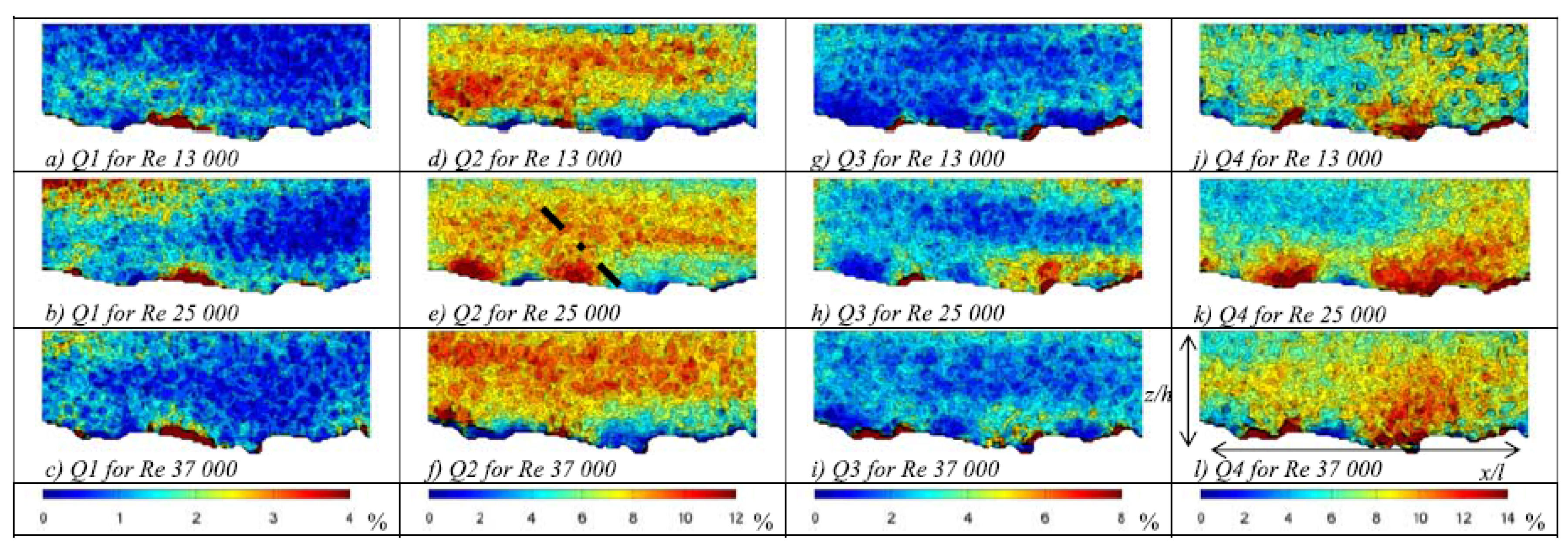
Quadrant analysis of two-dimensional velocity fluctuations (u′ and w′) is usually performed to understand the dynamics of the coherent flow structure in a turbulent flow. In general, in a turbulent boundary-layer flow, the turbulent events generated from the second and the fourth quadrants, termed ejections Q₂ (−u′ and +w′) and sweeps Q₄ (+u′ and −w′), respectively, are the dominating events, which govern the turbulence mechanism in the flow. On the other hand, those generated from the first and the third quadrants, termed outward interactions Q₁ (+u′ and +w′) and inward interactions Q₃ (−u′ and −w′), respectively, are the weak events, but they can be effective in the context of sediment entrainment [39].

In a WGB, Hardy et al. [27] performed the quadrant analysis to study the relative contribution from each event to the total Reynolds shear stress in governing the turbulent flow. As traditionally observed, their analysis also depicted that the sweeps in the near-bed flow zone are the prevailing events, while the ejections govern in the main flow layer. They however observed more localized flow patterns close to the bed. Near the bed, the ejections and sweeps occur in an alternative manner. In the leeside of a bed undulation, the sweeps govern the flow, while, in the stoss-side of the bed undulation, the ejections are ascendant, as shown in Figure 11. This suggests that the shape of the localized bed topography influences the turbulence characteristics. Furthermore, regarding the outward and inward interactions, they found that the occurrence of these events follows the alternative pattern, as observed for the sweeps and ejections. In the stoss-side of a particle, the outward interactions occur, while in the leeside of a particle, inward interactions prevail. Therefore, as the flow approaches the particle, it decelerates close to the bed; otherwise, it accelerates over or around the particle.

3.5. Effects of Water-Work on Secondary Currents

Turbulence driven secondary currents of Prandtl’s second kind are common in natural streams and arise in the flows in laboratory flumes as well [40], owing to anisotropy in turbulence. In this context, it is pertinent to mention that the secondary currents of Prandtl’s second kind are different from those of Prandtl’s first kind, which are governed by the streamline curvilinearity induced by the channel boundaries. Presence of secondary currents causes to redistribute the streamflow momentum. The secondary currents are more prominent in a narrow channel, for which the aspect ratio (channel width to flow depth ratio) is less than or equal to 5 [29,40]. On the other hand, in a wide channel having an aspect ratio greater than 5, the flow is deemed to be a two-dimensional with minimal effects of secondary currents at the central portion of flow in a channel [41]. Nevertheless, the secondary currents form cells in both narrow and wide channels.

To study the secondary currents in a WGB, McLelland [42] analyzed the flow characteristics in a WGB for three aspect ratios, such as 5, 10 and 20. They argued that the depth-averaged streamwise velocity could vary about ±5% along the channel cross-section, confirming the existence of secondary currents. The secondary currents forming cells across the channel width have similar dimensions as those along the flow depth and cause the redistribution of mean flow velocity and turbulent kinetic energy. In a WGB, the vectors of secondary currents show the dominance of the vortex with strong counterclockwise motion toward the channel wall-corner and the near-bed current toward the channel centerline. However, this observation in a WGB was fairly opposite to that found in an SGB, where the surface vortex is dominant. Comparing the results of all the aspect ratios, McLelland [42] found that the secondary current cell adjacent to the corner cells for a narrow channel is weaker than those in the intermediate (aspect ratio = 10) and wide channels (aspect ratio = 20). Additionally, in a wide channel, the secondary cells were observed to be stronger in the central portion of the channel. In all the cases, although the flow depth was kept identical for all the aspect ratios, the secondary current cells are of the order of the flow depth, inferring that the bed topography is not solely responsible for the size of secondary current cells. However, it is mainly responsible for the local modifications of the vectors of secondary currents.

4. Conclusions

This article presents the state-of-the-art research on WGBs, highlighting the impact of water-work on the bed topography and the turbulence characteristics. The water-work causes a difference in bed topography between a WGB and an SGB, even for an identical particle-size distribution in both the beds. The orientation as well as the alignment of surface particles in a WGB are adjusted by the flow in such way that the friction angles between the particles are smaller than those in an SGB. Moreover, analysis of the probability distribution function of the bed topographies revealed that the bed roughness structure in a WGB is positively skewed irrespective of sediment feeding rate, discharge and bed mobility conditions. Second- and higher-order structure functions show that a WGB possesses a higher correlation length scale than an SGB, confirming that the former has larger scale bed features than the latter. In addition, the Hurst coefficient in a WGB is higher than that in an SGB, indicating that the roughness structure in the former is more complex than that in the latter.

In the near-bed flow zone, the streamwise velocity in a WGB is more streamlined than that in an SGB owing to the better organized roughness structure in the former than in the latter, wherein they are randomly poised. Additionally, Reynolds and form-induced stresses revealed that the shapes of the turbulence stress profiles are independent of discharge, but dependent on the roughness and relative submergence. Quadrant analysis of turbulent events in WGBs infers that they are governed by the localized bed topography. Further, owing to the presence of the strong secondary currents, the flow cannot be considered as two-dimensional in a WGB, even for a wide channel. Besides, in a WGB, the bottom vortex dominates the flow, while in an SGB, the flow is mainly dominated by the surface vortex.

In essence, owing to the water-work, the roughness structures in WGBs are different from those in SGBs. The order of magnitude of bed roughness as well as turbulence characteristics are also higher in WGBs than in SGBs. Therefore, to obtain accurate results, it is necessary to perform laboratory experiments in WGBs, which resemble natural gravel-bed streams, rather than in SGBs. In addition, the existing results in SGBs are required to be treated carefully, if they are used to predict the resistance to flow, sediment transport, etc. Besides, regarding the scale-effects, in a laboratory experimental study, maintaining the similitude of some of the parameters (such as flow depth, flow velocity, gravel size, roughness, etc.) of the prototype with those of the model is a difficult proposition, as the conditions are often dissimilar. Thus, most experimental models dealing with gravel-bed are analyzed as distorted models, and the question of the applicability of the laboratory experimental results to prototype cases arises. However, Dey [40] and Novak et al. [43] described methods of analyzing the model results of rivers by taking into account the appropriate distortions in the scale ratios of various parameters. Finally, future research should also focus on obtaining corroborating data from prototypes to confirm the scalability of the laboratory results.

References

- Bathurst, J.C. Theoretical aspects of flow resistance. In Gravel-Bed Rivers; Hey, R.D., Bathurst, J.C., Thorne, C.R., Eds.; John Wiley: New York, NY, USA, 1985; pp. 83–108. [Google Scholar]
- Bray, D.I. Flow resistance in gravel-bed rivers. In Gravel-Bed Rivers; Hey, R.D., Bathurst, J.C., Thorne, C.R., Eds.; John Wiley: New York, NY, USA, 1985; pp. 109–132. [Google Scholar]
- Hey, R.D.; Thorne, C.R. Stable channels with mobile gravel beds. J. Hydraul. Eng. 1986, 112, 671–689. [Google Scholar] [CrossRef]
- Furbish, D.J. Conditions for geometric similarity of coarse streambed roughness. Math. Geol. 1987, 9, 291–307. [Google Scholar] [CrossRef]
- Kirchner, J.W.; Dietrich, W.E.; Iseya, F.; Ikeda, H. The variability of critical shear stress friction angle, and grain protrusion in water-worked sediments. Sedimentology 1990, 37, 647–672. [Google Scholar] [CrossRef]
- Robert, A. Boundary roughness in coarse-grained channels. Prog. Phys. Geogr. 1990, 14, 42–70. [Google Scholar] [CrossRef]
- Carling, P.A.; Kelsey, A.; Glaister, M.S. Effect of bed roughness, particle shape and orientation on initial motion criteria. In Dynamics of Gravel-Bed Rivers; Billi, P., Hey, R.D., Throne, C.R., Tacconi, P., Eds.; John Wiley: New York, USA, 1992; pp. 23–38. [Google Scholar]
- Nikora, V.; Goring, D.; Biggs, B.J.F. On gravel-bed roughness characterization. Water Resour. Res. 1998, 34, 517–527. [Google Scholar] [CrossRef]
- Marion, A.; Tait, S.J.; McEwan, I.K. Analysis of small-scale gravel bed topography during armoring. Water Resour. Res. 2003, 39, 1334. [Google Scholar] [CrossRef]
- Aberle, J.; Nikora, V. Statistical properties of armored gravel bed surfaces. Water Resour. Res. 2006, 42, W11414. [Google Scholar] [CrossRef]
- Buffin-Bélanger, T.; Rice, S.; Reid, I.; Lancaster, J. Spatial heterogeneity of near-bed hydraulics above a patch of river gravel. Water Resour. Res. 2006, 42, W04413. [Google Scholar] [CrossRef]
- Cooper, J.R.; Tait, S.J. Water-worked gravel beds in laboratory flumes: A natural analogue? Earth Surf. Proc. Land. 2009, 34, 384–397. [Google Scholar] [CrossRef]
- Monin, A.S.; Yaglom, A.M. Statistical Fluid Mechanics: Mechanics of Turbulence; MIT Press: Cambridge, MA, USA, 1975. [Google Scholar]
- Goring, D.; Nikora, V.; McEwan, I.K. Analysis of the texture of gravel beds using 2-D structure functions. In Proceedings of the IAHR Symposium on River, Coastal, and Estuarine Morphodynamics, Guona, Italy; Seminara, G., Blondeaux, P., Eds.; Springer: New York, NY, USA, 1999; Volume 2, pp. 111–120. [Google Scholar]
- Butler, J.B.; Lane, S.N.; Chandler, J.H. Characterization of the structure of river-bed gravels using two-dimensional fractal analysis. Math. Geol. 2001, 33, 301–330. [Google Scholar] [CrossRef]
- Qin, J.; Ng, S.L. Multifractal characterization of water-worked gravel surfaces. J. Hydraul. Res. 2011, 49, 345–351. [Google Scholar] [CrossRef]
- Nikora, V.; Walsh, J. Water-worked gravel surfaces: High-order structure functions at the particle scale. Water Resour. Res. 2004, 40, W12601. [Google Scholar] [CrossRef]
- Davis, A.; Marshak, A.; Wiscombe, W.; Cahalan, R. Multifractal characterizations of nonstationarity and intermittency in geophysical fields: Observed, retrieved, or simulated. J. Geophys. Res. 1994, 99, 8055–8072. [Google Scholar] [CrossRef]
- Frisch, U. Turbulence: The Legacy of A. N. Kolmogorov; Cambridge University Press: New York, NY, USA, 1995. [Google Scholar]
- Kolmogorov, A.N. Local structure of turbulence in an incompressible fluid for very large Reynolds numbers. Dokl. Akad. Nauk SSSR 1941, 30, 299–303. [Google Scholar] [CrossRef]
- Alen, J.R.L. Sedimentary Structures: Their Character and Physical Basis; Elsevier: New York, NY, USA, 1982. [Google Scholar]
- Smart, G.M.; Aberle, J.; Duncan, M.; Walsh, J. Measurement and analysis of alluvial bed roughness. J. Hydraul. Res. 2004, 42, 227–237. [Google Scholar] [CrossRef]
- Bergeron, N.E. Scale-space analysis of stream-bed roughness in coarse gravel-bed streams. Math. Geol. 1996, 28, 537–561. [Google Scholar] [CrossRef]
- Barison, S.; Chegini, A.; Marion, A.; Tait, S.J. Modifications in near bed flow over sediment beds and the implications for grain entrainment. In Proceedings of the 30th IAHR Congress, Thessalonki, Greece, 24–29 August 2003; pp. 509–516. [Google Scholar]
- Cooper, J.R.; Tait, S.J. The spatial organisation of time-averaged streamwise velocity and its correlation with the surface topography of water-worked gravel beds. Acta Geophys. 2008, 56, 614–642. [Google Scholar] [CrossRef]
- Legleiter, C.J.; Phelps, T.L.; Wohl, E.E. Geostatistical analysis of the effects of stage and roughness on reach-scale spatial patterns of velocity and turbulence intensity. Geomorphology 2007, 83, 322–345. [Google Scholar] [CrossRef]
- Hardy, R.J.; Best, J.L.; Lane, S.N.; Carbonneau, P.E. Coherent flow structures in a depth-limited flow over a gravel surface: The role of near-bed turbulence and influence of Reynolds number. J. Geophys. Res. 2009, 114, F01003. [Google Scholar] [CrossRef]
- Koll, K.; Cooper, J.R.; Aberle, J.; Tait, S.J.; Marion, A. Investigation into the physical relationship between water-worked gravel bed armours and turbulent in-channel flow patterns. In Proceedings of the HYDRALAB III Joint User Meeting, Hannover, Germany, February 2010. [Google Scholar]
- Nezu, I.; Nakagawa, H. Turbulence in Open-Channel Flows; CRC Press: Rotterdam, The Netherlands, 1993. [Google Scholar]
- Pu, J.H.; Wei, J.; Huang, Y. Velocity distribution and 3d turbulence characteristic analysis for flow over water-worked rough bed. Water 2017, 9, 668. [Google Scholar] [CrossRef]
- Dey, S.; Raikar, R.V. Characteristics of loose rough boundary streams at near-threshold. J. Hydraul. Eng. 2007, 133, 288–304. [Google Scholar] [CrossRef]
- Padhi, E.; Penna, N.; Dey, S.; Gaudio, R. Hydrodynamics of water-worked and screeded gravel beds: A comparative study. Phys. Fluids 2018, 30, 085105. [Google Scholar] [CrossRef]
- Nikora, V.; McLean, S.; Coleman, S.; Pokrajac, D.; McEwan, I.; Campbell, L.; Aberle, J.; Clunie, D.; Koll, K. Double-averaging concept for rough bed open-channel and overland flows: Applications. J. Hydraul. Eng. 2007, 133, 884–895. [Google Scholar] [CrossRef]
- Aberle, J.; Koll, K.; Dittrich, A. Form induced stresses over rough gravel-beds. Acta Geophys. 2008, 56, 584–600. [Google Scholar] [CrossRef]
- Cooper, J.R.; Tait, S.J. Spatially representative velocity measurement over water-worked gravel beds. Water Resour. Res. 2010, 46, W11559. [Google Scholar] [CrossRef]
- Cooper, R.; Aberle, J.; Koll, K.; Tait, S.J. Influence of relative submergence on spatial variance and form-induced stress of gravel-bed flows. Water Resour. Res. 2013, 49, 5765–5777. [Google Scholar] [CrossRef]
- Mignot, E.; Barthelemy, E.; Hurther, D. Double-averaging analysis and local flow characterization of near-bed turbulence in gravel-bed channel flows. J. Fluid. Mech. 2009, 618, 279–303. [Google Scholar] [CrossRef]
- Dey, S.; Das, R. Gravel-bed hydrodynamics: Double-averaging approach. J. Hydraul. Eng. 2012, 138, 707–725. [Google Scholar] [CrossRef]
- Nelson, J.M.; Shreve, R.L.; McLean, S.R.; Drake, T.G. Role of near-bed turbulence structure in bed load transport and bed form mechanics. Water Resour. Res. 1995, 31, 2071–2086. [Google Scholar] [CrossRef]
- Dey, S. Fluvial Hydrodynamics: Hydrodynamic and Sediment Transport Phenomena; Springer-Verlag: Berlin, Germany, 2014. [Google Scholar]
- Nikora, V.; Roy, A.G. Secondary flows in rivers: Theoretical framework, recent advances, and current challenges. In Gravel Bed Rivers: Processes, Tools, Environments; Church, M., Biron, P.M., Roy, A.G., Eds.; John Wiley & Sons Ltd: Chichester, UK, 2012; pp. 3–22. [Google Scholar]
- McLelland, S.J. Coherent secondary flows over a water-worked rough bed in a straight channel. In Coherent Flow Structures at Earth’s Surface; Venditti, J.G., Best, J.L., Church, M., Hardy, R.J., Eds.; John Wiley & Sons Ltd: Chichester, UK, 2013; pp. 275–288. [Google Scholar]
- Novak, P.; Cabelka, J. Models in Hydraulic Engineering; Pitman: London, UK, 1981. [Google Scholar]
Figure 1.
Photograph of a natural gravel-bed stream with a flow direction right to left (a); and close view of the natural gravel-bed stream with a flow direction left to right (b).
Figure 2.
Photograph of an SGB in a laboratory flume (a); and a close view (b).
Figure 3.
Probability density functions of bed surface fluctuations with respect to the mean surface level in WGBs (namely, Fed bed 1, Fed bed 2, and Fed bed 3) and an SGB (data extracted from Cooper and Tait [12]).
Figure 4.
Non-dimensional structure function of a WGB (data extracted from Nikora and Walsh [17]).
Figure 5.
Variations of scaling exponents ξ of the generalized structure function with the order p (data extracted from Nikora and Walsh [17]).
Figure 6.
Contours of the second-order structure function for the roughness structure at a discharge of 0.25 m3 s−1 (data extracted from Aberle and Nikora [10]).
Figure 7.
Variations of non-dimensional streamwise velocity with non-dimensional vertical distance zu*/ν and (z + Δz)/ks in smooth and rough beds (WGB and SGB), respectively (data extracted from Pu et al. [30]).
Figure 8.
Variations of non-dimensional DA streamwise velocity with non-dimensional vertical distance (z + Δz)/Δz in the WGB and SGB. The red and blue broken lines indicate the form-induced sublayers in the WGB and SGB, respectively (data extracted from Padhi et al. [32]).
Figure 9.
Variations of non-dimensional SA Reynolds shear stress 〈〉/ and SA form-induced shear stress 〈τf〉/ with non-dimensional vertical distance z/h in the WGB and SGB (data extracted from Padhi et al. [32]).
Figure 10.
Variations of SA form-induced normal stress 〈σfuu〉 (=〈〉/ρ) with z–z0 in the WGB (data extracted from Aberle et al. [34]).
Figure 11.
Flow structures as examined with the quadrant analysis: (a–c) first quadrant (outward intersections); (d–f) second quadrant (ejections); (g–i) third quadrant (inward intersections); and (j–l) fourth quadrant (sweeps) (data extracted from Hardy et al. [27]).
© 2019 by the authors. Licensee MDPI, Basel, Switzerland. This article is an open access article distributed under the terms and conditions of the Creative Commons Attribution (CC BY) license (http://creativecommons.org/licenses/by/4.0/).
Share and Cite
MDPI and ACS Style
Padhi, E.; Dey, S.; Desai, V.R.; Penna, N.; Gaudio, R. Water-Worked Gravel Bed: State-of-the-Art Review. Water 2019, 11, 694. https://doi.org/10.3390/w11040694
AMA Style
Padhi E, Dey S, Desai VR, Penna N, Gaudio R. Water-Worked Gravel Bed: State-of-the-Art Review. Water. 2019; 11(4):694. https://doi.org/10.3390/w11040694
Chicago/Turabian StylePadhi, Ellora, Subhasish Dey, Venkappayya R. Desai, Nadia Penna, and Roberto Gaudio. 2019. "Water-Worked Gravel Bed: State-of-the-Art Review" Water 11, no. 4: 694. https://doi.org/10.3390/w11040694
Note that from the first issue of 2016, this journal uses article numbers instead of page numbers. See further details here.