Estimation of Hydrologic Alteration in Kaligandaki River Using Representative Hydrologic Indices

Abstract

Anthropogenic activities have led to the transformation of river basins and natural flow alteration around the world. Alteration in flow regimes have adverse effects on river ecosystems. Flow value changes signify the alteration extent and a number of flow related indices can be used to assess the extent of alteration in a river ecosystem. Selection of a few and ecologically relevant indices from a large set of available indices is a daunting task. Principal Component Analysis helps to reduce these large indices to a few ecologically significant indices and removes statistical redundancy of data to give uncorrelated data sets. These representative indices are useful in the primary investigation of a less studied area like the Kaligandaki River basin, Nepal. This paper uses reduced indices from the Kaligandaki River to calculate the alteration on the river section downstream of a hydropower facility using the Histogram Comparison Approach (HCA) combined with Hydrologic Year Types (HYT). The combined approach eliminates the potential underestimation of alteration values which may occur due to the exemption of hydrologic year types from the analysis, a feature equally relevant in river ecology. A new metric is used for the calculation of combined alteration using HCA-HYT in this paper. The analysis showed 60.71 percent alteration in the natural flow regime in the area past a hydropower construction, which is classified in the high alteration category. The study can be a guide for further analysis of the ecological flow management of a river section and a parsimonious approach to other areas where hydrological data is limited to historical flow records only.

1. Introduction

Rivers are integral parts of human civilization and ecosystems in their own right, with their health depending on the flow regime characteristics [1,2,3]. Flow has been pointed out as a “master variable” in river ecosystems, and its alteration due to river regulation projects disturbs the natural flow regime, which in turn degrades the ecological integrity of the river ecosystem [4,5,6,7,8]. The direct link of flow regime characteristics with the ecological attributes are of prime concern for the solid foundation of eco-hydrology [9,10]. While this direct link establishment is a mammoth task, various ecological linkages of flow parameters have been intensively studied while considering broader ecological consequences [1,11,12,13,14] Quantifying the flow regime for proper flow management considering ecological consequences has promoted the development of various hydrologic indicators [15]. Earlier practices of assigning a single minimum flow standard to maintain the river ecology have been proven to be insufficient as rivers hold diverse species and single flow settings favor the single species in consideration [1,11,14,16,17,18,19,20,21]. The concept of flow variability later replaced this single flow approach, whereby the natural variability in the flow of the river has been attributed to the healthy functioning of the river ecosystem [16,17]. Variation of flow in terms of magnitude, frequency, timing, duration, and rate is commonly used to represent the temporal variation in the river. Close maintenance of the temporal flow variation in the river to “natural flow variability” has been accepted as a necessary criteria to minimize environmental impacts on the altered river ecosystem [16,17,19]. The main challenge here is to quantify the level of flow variations after the natural period.

RVA (Range of Variability Approach) is one of the earliest methods used to calculate flow variation of the river in terms of magnitude, frequency, timing, duration, and the rate of change of flow events. The 33 Indicators of Hydrologic Alteration represented these five terms (IHA) [16]. On the basis of the frequency difference of IHAs falling within the target range between the natural and altered period, the alteration is measured [14,17,21]. IHA indices or parameters single-handedly captured the majority of the variation and information that is provided by the most widely used 171 indices worldwide, making it a formidable choice for representing the alteration in rivers [15]. The RVA method, however, does not consider the variation of parameters falling within the target range and those outside the range, sometimes seriously underestimating the degree of alteration [22]. Using IHA indices, the Histogram Matching Approach (HMA) and its subsequent extension Histogram Comparison Approach (HCA), we considered the alteration on whole flow regime, unlike the RVA approach which only considered alteration within a predefined target range [22,23]. Furthermore, HCA performed better than HMA in providing judgment on alteration because it considered cross-class correspondence in addition to class-by-class correspondence [23]. HCA also considered the alteration related to the hydrologic year types (HYT) i.e., wet, average and dry years, however, it failed to consider the alteration of their order. The HYT order change in flow regimes due to anthropogenic causes is as important as other indices, as for some species this order has been found to be more important than events within individual years [24]. Long term operation of reservoirs particularly requires the incorporation of scenarios related to hydrologic year types in flow release decisions [25]. A holistic approach is thus necessary to consider alteration within a year and in an order of years. This can be achieved by combining the metrics related to HCA and HYT to give a single metric. A new formula associated with this combined metric is used in this paper. Further studies showed that many of the indices used in IHA are intercorrelated, thus increasing their statistical redundancy [9,15,26]. The use of a small number of these indices in the ecological objective of flow optimization problems reduces both computational efforts and costs in numerical applications [9,10,20,27]. Principal Component Analysis (PCA) is an effective statistical method to retain the non-redundant indices. Although PCA is defined originally for data with multi-normal distribution, moderately skewed data deviated from normality do not bias the analysis [28]. IHA indices unlike original historic flow data do not directly confirm to a non-normal distribution [29]. The indices derived from PCA are useful in future environmental flow management decisions [30,31].

This paper uses IHA based RVA and HCA methods in the Kaligandaki River to calculate the flow regime alteration after construction of a hydropower facility. These results are then compared with each other, then after combined with alteration results from the HYT method to give a final comprehensive flow regime alteration value for the river. The IHA indices are subjected to Principal Component Analysis and statistically non-redundant sets of reduced IHA indices are obtained for the river section. These indices are used to calculate the new alteration values for RVA and HCA methods as well as being combined with HYT to give a final combined flow regime alteration value. The results for final alteration calculated with full indices sets of IHA and reduced indices set obtained from PCA are compared. The main objective of the paper is to present the new combined approach for the calculation of the hydrological alteration and obtain reduced indices that can fully represent the hydrologic variability of the river. The current practice of single minimum flow release policy in the Kaligandaki River is not suitable for the sustainability of the river in the long run [32]. The projects expected in the future require proper research guidelines related to hydro-ecology for defining environmental flow settings. The basic step in defining environmental flow requirements is firsthand assessment of the hydrologic alteration. For areas like the Kaligandaki River Basin where data and costs are constraints, the method explained here can be used as a parsimonious approach to calculate comprehensive hydrologic alteration. The obtained results can be used by concerned stakeholders as the basis for the ecological management of rivers in the basin.

2. Materials and Methods

2.1. Study Area

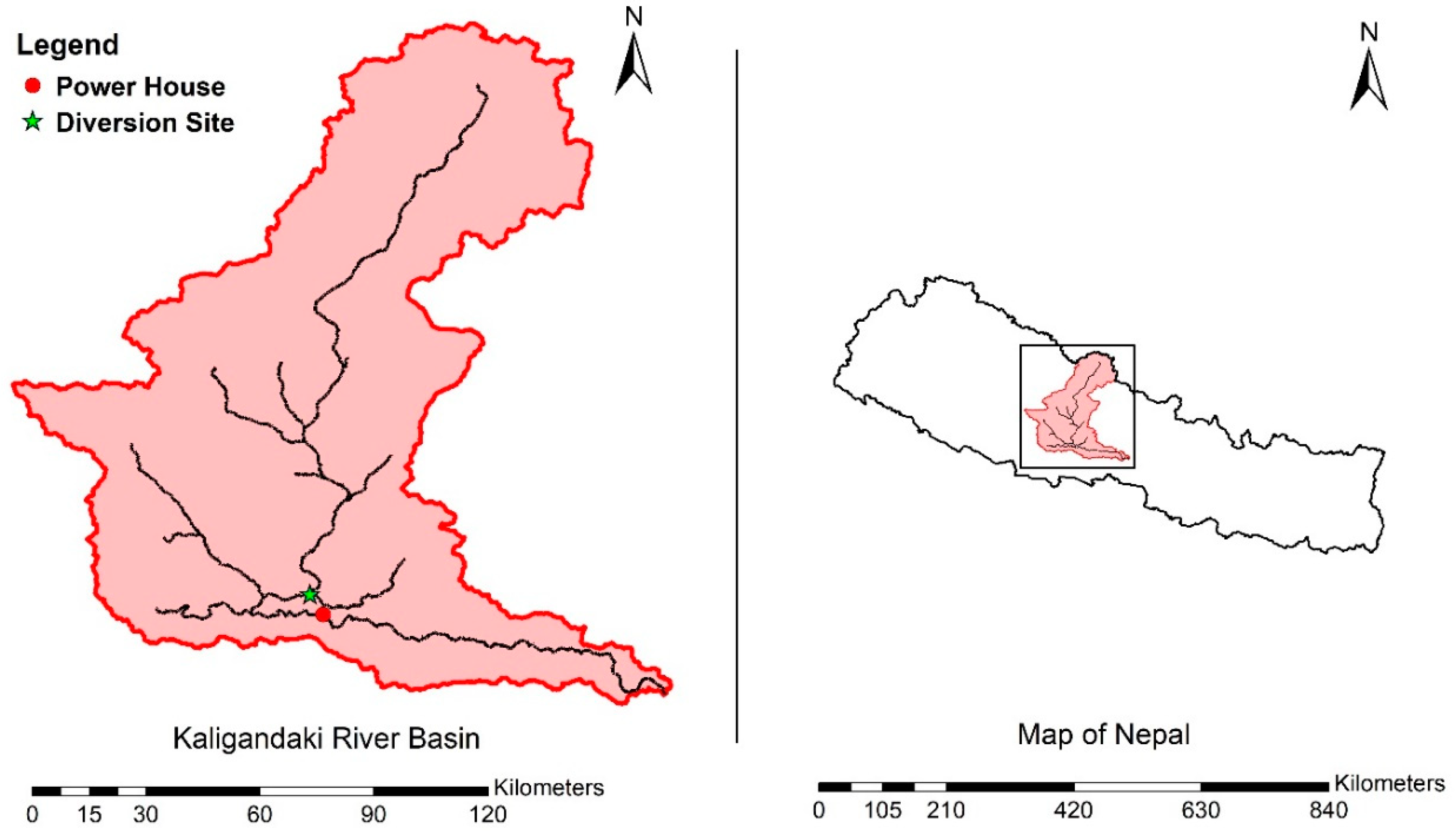
Kaligandaki is one of the major rivers of Nepal and is also the main tributary of Narayani River, which later joins the Ganges in India as a left bank tributary. Kaligandaki River basin (Figure 1) has an elevation range of 190 m to 8168 m MSL (above mean sea level). It has a total catchment area of 11,851 sq. km and lies between 82$°$52.8′ E to 84$°$26.3′ E and 27$°$43.2′ N to 29$°$19.8′ N.

The mean annual precipitation in the river basin is 1396mm with high spatial variation. 80% of this precipitation value occurs during the wet monsoon season (June–August) [33,34]. Annual flow for the river can be divided into three categories based on percentiles of long term mean monthly flow (

Table 1. Mean monthly flow and flow classification for the Kaligandaki River.

Month	Mean Flow (cms)	Flow Category
January	88.13	Intermediate
February	75.58	Low
March	68.47	Low
April	66.58	Low
May	130.7	Intermediate
June	164.7	Intermediate
July	1119	High
August	1376	High
September	1032	High
October	468.5	Intermediate
November	233.3	Intermediate
December	151.8	Intermediate

Note: cms (cubic meters per second).

). Flows below 25th percentile are classified as low flows, above 75th percentile classified as high flow, whereas between 25th and 75th percentile are defined as intermediate flows. Kaligandaki River is a high sediment-laden river with suspended sediment of 43 Mt/year. A hydropower station was constructed in Syangja district with a generating capacity of 144MW under a run-of-river scheme by diverting the river through a tunnel with a length of 6 km. The power plant operates in a peaking scheme during the dry season, thereby causing a significant impact on low flow values downstream. The hydrological station used in the analysis is about 12 km upstream of confluence between Kaligandaki and Narayani. The river is home to diverse aquatic life (mostly freshwater fish) and plants throughout the basin area.

Hydrological data from the periods of 1983–1996 and 2002–2015 were obtained from the Department of Hydrology and Meteorology, Nepal. The water year for Nepal starts from the first of July. The construction of hydropower project began in 1996 and was completed in 2002. This period thus marked the pre-impact and post-impact period. The RVA and HCA method used the daily flow from the pre-impact period (1983–1996) and post-impact period (2002–2015). The HYT method meanwhile used the annual average flow for the same two periods. Calculation of hydrologic alteration for each of the 33 indices based on RVA method is performed using IHA Software (https://www.conservationgateway.org/) [14,35]. Only 32 indices were taken into account as there is no zero-day flow recorded in the station.

2.2. Methods

2.2.1. Principal Component Analysis (PCA)

PCA is a multivariate data analytic technique which reduces the dimensionality of interrelated variables in a data set to extract important information represented by a set of new uncorrelated orthogonal variables [28,36,37]. Correlation matrix for PCA is calculated using values from 32 parameters of IHA analyzed by the software. Eigenvalues from a 32-by-32 correlation matrix for Pearson and Spearman methods are used to extract Principal Components (PCs) [28]. These principal components are orthogonal to each other and are arranged in the descending order based on the amount of variance of data explained. The retention of meaningful components is done on the basis of the Kaiser-Guttman Criteria, which retains PC with an eigenvalue loading higher than 1.0 (λ > 1.0) [26,31,38]. Orthogonal rotation is done for the selection of subspaces from retained principal components. The total maximum variance of original subspace remains unchanged after rotation, but it is redistributed amongst the rotated components more evenly than before [39]. Orthogonal Varimax rotation proposed by Kaiser is used to get factor loadings [40]. A single variable with the highest absolute loadings on each of the selected PCs are used to represent the PC. Furthermore, variables with loadings within a range of ±0.5 are excluded from further analysis [41]. Since the number of IHA indices retained are still higher, Kaiser–Meyer–Olkin (KMO) Measure of Sampling Adequacy (MSA) is performed and only meritorious class indices are retained [31,41,42].

2.2.2. Histogram Comparison Approach (HCA)

The HCA method is based on class by class correspondence and cross-class correspondence of the information in data [23]. Histograms for 32 IHA indices are constructed and their frequency vectors are compared using two similarity metrics. Those two similarity metrics are combined to form a single similarity metric, which is used to calculate the dissimilarity and in turn the alteration. Alteration by the HCA method is discussed in detail by Huang et al. (2017) [23]. The overall degree of alteration is calculated using a group average technique as given by Xue et al. (2017) [43] and the final value is represented by “A”. The results for the final HCA alteration “A” lie in the range of [0, 1], zero being no alteration and 1 being 100% alteration with respect to pre-impact or the natural period. The pre-impact period of 1983–1996 and post-impact period of 2002–2015 are used to calculate the alteration values. An alteration value from a reduced set of indices by PCA method is also calculated.

2.2.3. Hydrologic Year Types (HYT)

The HYT method considers alteration in order of occurrence of certain hydrologic year types e.g., dry, average and wet years. It addresses the basic defects of RVA and HCA methods, which fail to consider the alteration of the order of hydrologic year types. Flow pulses are the basic indicators of river health and disturbances in order of such pulses may have adverse effects on some species relying on them [15,24,44]. Detailed calculation of alteration from the HYT method is given by Yin et al. (2015) [24] and the final value is represented by “A*”. “A*” is the alteration value in the order of hydrologic year types. The range of “A*” lies within [0, 1], 0 being no alteration and 1 being 100% alteration in a flow regime in the post-impact period as compared to the pre-impact period.

2.2.4. Combined Alteration using HCA and HYT

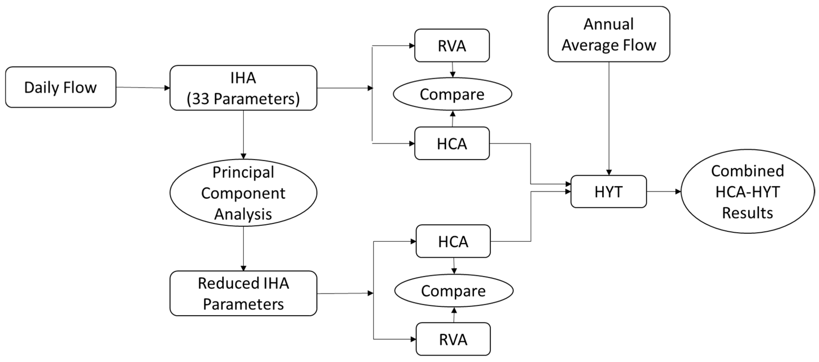
To address the shortcomings of HCA in underestimating alteration, HYT is combined with HCA to give a new metric of alteration [24]. This metric gives the overall alteration of the river in frequency, magnitude, timing, the rate of change of flow events, hydrologic year types and order of hydrologic year types. The combined overall degree of alteration is given by the new formula:

$$K=1-\sqrt{\left[\left(1-A\right)\times \left(1-A^{*}\right)\right]}$$

(1)

The value of K lies between [1, 0]. Thus, this method gives a refined value of alteration on the river and since takes into account for alteration due to HYT and HCA, it gives a broader and reliable value. The whole calculation process is present in the Figure 2 given below.

3. Results

3.1. Principal Component Analysis

The end result of principal component analysis is the non-redundant subset selection, as explained below in detail.

3.1.1. Scree Plot of Eigenvalues and PCA Subset Selection

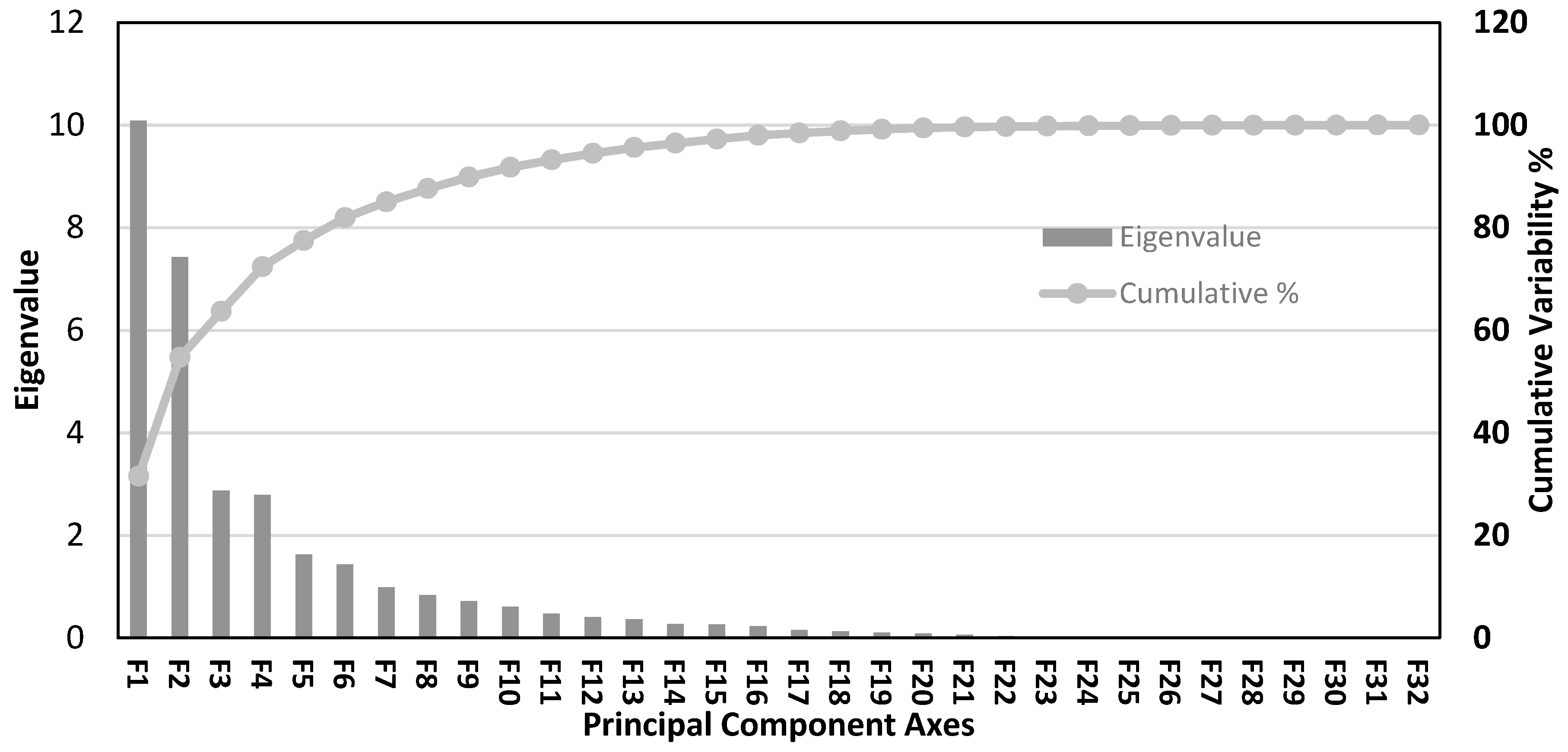
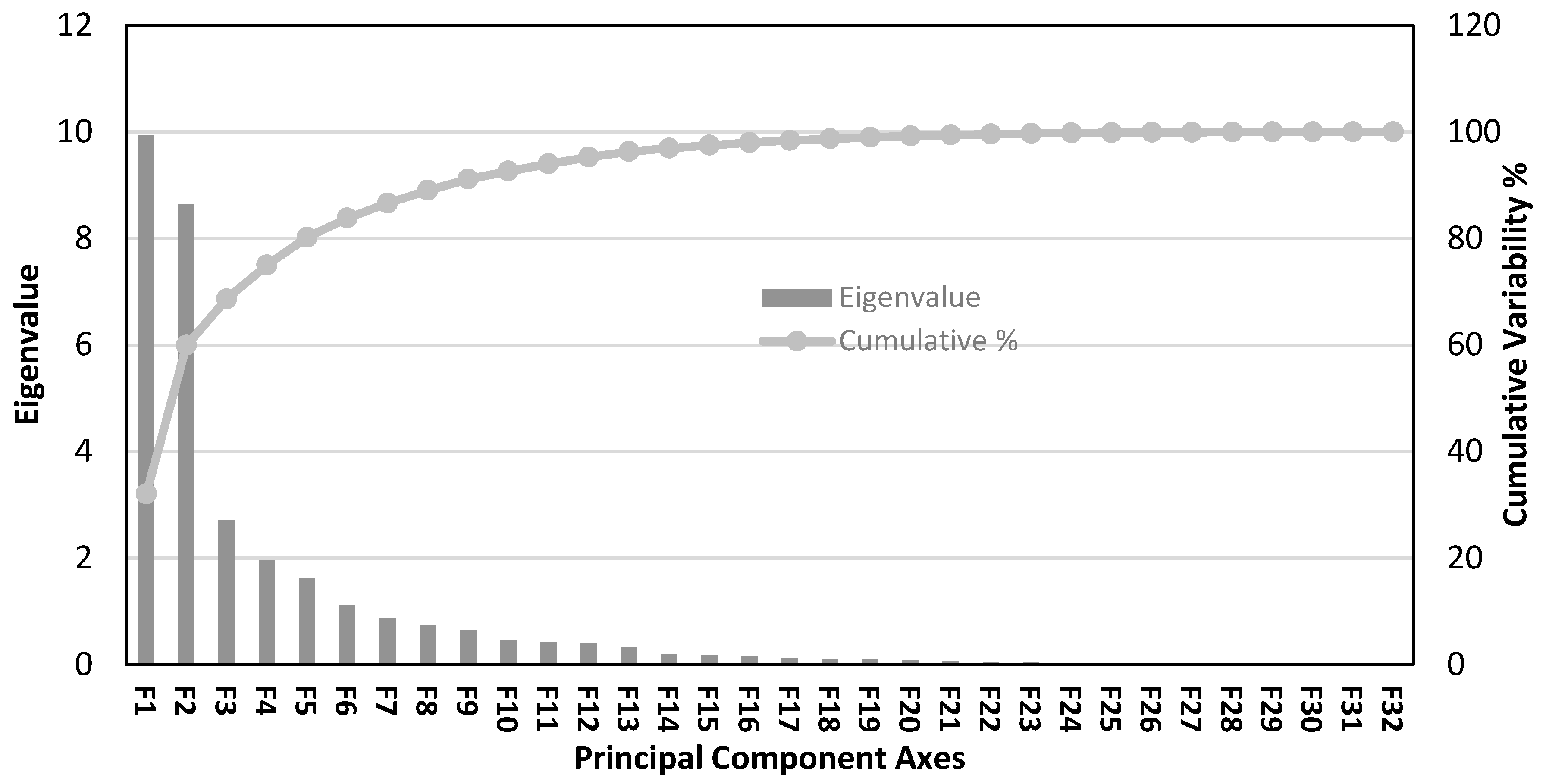
The 32 principal component axis associated with the original data are represented by F1, F2, …, F32. Variance in PCA axis is directly proportional to its associated eigenvalue, with higher eigenvalues corresponding to the higher variance explained in that axis. A lower eigenvalue explains little variance in data, thus axes with higher eigenvalues are selected to represent the whole flow regime in both the Pearson and Spearman’s Method. Figure 3 and Figure 4 shows the scree plot for both methods with the highest eigenvalue for component F1 and decreasing gradually for the next ones.

Six PC axes with eigenvalues greater than 1.0 are selected for both methods. These selected axes explain 81.96% and 83.79% of the total variability in Pearson and Spearman’s method, respectively (

Table 2. Eigenvalue with variability and cumulative variability for selected PC axes from Pearson and Spearman’s method.

Pearson Method				Spearman’s Method
PC Axes	Eigenvalue	Variability (%)	Cumulative %	PC Axes	Eigenvalue	Variability (%)	Cumulative %
F1	10.08	31.51	31.51	F1	9.93	32.04	32.04
F2	7.43	23.21	54.71	F2	8.64	27.87	59.91
F3	2.87	8.98	63.69	F3	2.70	8.72	68.63
F4	2.79	8.71	72.40	F4	1.96	6.34	74.97
F5	1.62	5.07	77.47	F5	1.62	5.24	80.21
F6	1.44	4.49	81.96	F6	1.11	3.58	83.79

). The factor loadings for data points on each axis are presented in

Table 3. Loadings for first Six PCs in the Pearson Method.

Parameters	F1	F2	F3	F4	F5	F6
June	−0.123	0.446	−0.169	−0.116	−0.108	0.558
July	−0.266	0.524	−0.003	−0.426	0.218	0.503
August	−0.590	0.488	0.069	−0.384	0.058	−0.066
September	−0.413	0.394	0.034	0.384	−0.026	−0.258
October	−0.175	0.440	0.151	0.626	−0.099	−0.234
November	−0.141	0.605	−0.058	0.663	0.118	0.036
December	0.111	0.500	−0.112	0.533	0.147	0.188
January	0.762	0.388	−0.239	−0.037	−0.160	−0.106
February	0.827	0.348	−0.231	−0.121	−0.132	−0.122
March	0.864	0.368	−0.145	−0.094	−0.136	−0.106
April	0.862	0.359	−0.080	−0.134	−0.235	−0.079
May	0.628	0.362	0.105	−0.220	−0.377	−0.100
1-day min	0.557	0.384	0.669	0.093	−0.027	0.248
3-day min	0.633	0.400	0.595	0.067	0.096	0.213
7-day min	0.692	0.386	0.538	0.041	0.140	0.176
30-day min	0.815	0.472	0.074	0.081	0.118	0.083
90-day min	0.858	0.463	−0.089	−0.001	0.005	0.011
1-day max	−0.398	0.769	−0.037	0.014	0.006	−0.228
3-day max	−0.453	0.749	0.152	−0.013	0.008	−0.192
7-day max	−0.510	0.777	0.104	−0.083	0.030	−0.035
30-day max	−0.627	0.664	0.134	−0.257	0.050	−0.027
90-day max	−0.599	0.733	0.087	−0.147	0.107	0.073
Base flow	0.822	−0.308	0.402	0.001	0.089	0.025
Date min	−0.388	−0.108	−0.177	0.158	0.602	0.205
Date max	−0.361	−0.108	0.445	0.673	−0.035	−0.091
Low pulse count	0.640	0.116	−0.398	−0.027	0.443	−0.214
Lo pulse Duration	−0.514	−0.112	−0.278	0.029	−0.491	0.375
High pulse Count	0.396	−0.017	−0.586	0.472	−0.013	0.342
High pulse Duration	−0.363	0.443	0.159	−0.483	0.112	−0.190
Rise rate	−0.325	0.744	−0.299	0.104	−0.300	0.017
Fall rate	−0.126	−0.741	0.545	−0.091	−0.017	0.009
Number of Reversals	0.508	0.096	−0.323	−0.142	0.534	−0.151
Axis Interpretation	Low to Intermediate flow, Minimum flow, Base flow	Maximum flow, High flow month, Rise	Mix	Intermediate flow month, Date of maximum flow	Mix	High Flow Month

Note: Value in bold italics corresponds to highest loading in that PC.

and

Table 4. Loadings for first Six PCs in Spearman’s Method.

Parameters	F1	F2	F3	F4	F5	F6
June	0.072	0.400	−0.109	0.531	−0.148	0.309
July	−0.012	0.592	−0.308	0.215	0.196	0.540
August	−0.311	0.688	−0.311	−0.128	0.081	−0.130
September	−0.224	0.541	0.324	−0.250	−0.120	0.122
October	−0.085	0.527	0.670	−0.046	−0.005	−0.047
November	0.104	0.603	0.668	−0.086	0.104	−0.059
December	0.392	0.537	0.498	−0.126	0.044	−0.034
January	0.755	0.373	0.252	−0.136	0.133	0.080
February	0.882	0.212	0.088	−0.030	0.244	0.075
March	0.949	0.158	−0.055	−0.059	0.096	0.035
April	0.877	0.119	−0.139	0.112	−0.182	−0.082
May	0.595	0.161	−0.185	0.295	−0.422	−0.251
1-day min	0.850	0.185	−0.080	−0.187	−0.294	0.220
3-day min	0.920	0.176	−0.104	−0.128	−0.172	0.142
7-day min	0.950	0.142	−0.086	−0.110	−0.110	0.108
30-day min	0.965	0.165	−0.048	−0.052	0.036	0.044
90-day min	0.965	0.205	−0.020	0.025	0.063	0.052
1-day max	−0.103	0.863	−0.040	0.087	0.015	−0.182
3-day max	−0.091	0.880	−0.090	−0.027	−0.069	−0.136
7-day max	−0.144	0.925	−0.091	−0.015	−0.083	−0.084
30-day max	−0.254	0.882	−0.267	−0.108	0.009	−0.043
90-day max	−0.227	0.916	−0.097	−0.044	0.023	0.145
Base flow	0.767	−0.554	−0.076	−0.156	−0.044	−0.018
Date min	−0.331	0.163	0.254	−0.333	0.566	0.297
Date max	−0.059	0.019	0.470	−0.515	−0.504	−0.153
Low pulse count	0.505	−0.202	−0.006	0.200	0.597	−0.374
Low pulse Duration	−0.858	−0.018	−0.066	−0.050	−0.320	0.269
High pulse Count	0.086	−0.242	0.681	0.539	−0.101	0.233
High pulse Duration	−0.127	0.650	−0.472	−0.456	0.086	−0.047
Rise rate	−0.181	0.804	0.099	0.348	−0.158	−0.073
Fall rate	−0.009	−0.735	−0.083	−0.507	−0.098	0.219
Number of Reversals	0.459	0.166	−0.313	−0.132	0.585	−0.242
Axis Interpretation	Low to intermediate flow months, Minimum Flow, Base Flow	High flow months, Maximum flow, High Pulse, Rise, fall duration	Intermediate flow months, High Pulse count	Mix	Mix	-

Note: Value in bold italics corresponds to the highest loading in that PC.

. The highlighted clusters in Table 3 and Table 4 indicate the dominant IHA groups for each axis and can be used to interpret the axis. For Pearson Method, first axis F1 is related to low-intermediate flow month, base flow and minimum flows. F2 is related to maximum flows, F3 and F5 meanwhile showed no particular dominance. F4 is related to the intermediate flow month and date of maximum flow, with F6 dominated by a single high flow month.

For Spearman’s method, F1 represents Low-Intermediate flow months, minimum flow values and base flow, whereas F2 is associated with high flow months, maximum flow, high pulse, and rise-fall rate. F3 is dominated by intermediate flow months and high pulse count, while the rest of the axis shows no particular clustering.

From Table 3 and Table 4, 30 common indices related to both the Pearson and Spearman’s method have been found, which are still higher. A KMO test for the measure of sampling adequacy is done to further reduce the number of indices, with a selection of the meritorious class only (

Table 5. IHA indices with meritorious class loadings for Pearson and Spearman’s method along with KMO test range classification.

Pearson Method			Spearman’s Method
Parameter	Loading	PC Axis	Parameter	Loading	PC Axis
February	0.827	F1	February	0.882	F1
March	0.864	F1	March	0.949	F1
April	0.862	F1	April	0.877	F1
30-day minimum	0.815	F1	1-day minimum	0.850	F1
90-day minimum	0.858	F1	3-day minimum	0.920	F1
Base Flow	0.822	F1	7-day minimum	0.950	F1
KMO Test			30-day minimum	0.965	F1
Loading Range	Class		90-day minimum	0.965	F1
0.00–0.49	Unacceptable		Low pulse duration	0.858	F1
0.50–0.59	Miserable		1-day Maximum	0.863	F2
0.60–0.69	Mediocre		3-day maximum	0.880	F2
0.70–0.79	Middling		7-day maximum	0.925	F2
0.80–0.89	Meritorious		30-day maximum	0.882	F2
0.90–1.00	Marvelous		90-day maximum	0.916	F2
			Rise rate	0.804	F2

).

Five common indices for both the Pearson and Spearman’s method are selected from Table 5 to represent the flow regime of the Kaligandaki River. These indices include IHA parameters of February mean monthly flow, March mean monthly flow, April mean monthly flow, 30-day minimum flow, and 90-day minimum flow. These parameters are used to compare alteration values between the reduced and full set of IHA parameters used in RVA and HCA methods.

3.1.2. The Alteration from RVA and HCA Methods

RVA results in

Table 6. Percentage alteration from RVA and HCA methods for the parameter of 5 IHA groups.

IHA Group 1	RVA	HCA	IHA Group 2	RVA	HCA	IHA Group 3	RVA	HCA
July	33.33	48.99	1-day minimum	10.00	50.51	Date minimum	−11.11	33.46
August	37.50	5.37	3-day minimum	−30.00	50.51	Date maximum	22.22	54.36
September	−30.00	47.51	7-day minimum	−50.00	50.60
October	−11.11	22.57	30-day minimum	−54.55	53.71	IHA Group 4
November	−10.00	21.75	90-day minimum	−50.00	60.66	Low pulse Count	−81.82	78.57
December	0.00	14.29	1-day maximum	50.00	29.72	Low pulse Duration	−8.33	57.14
January	0.00	21.43	3-day maximum	71.43	39.14	High pulse Count	−10.00	32.99
February	−22.22	59.96	7-day maximum	42.86	51.55	High pulse Duration	−12.50	28.57
March	−45.45	40.43	30-day maximum	−20.00	32.99
April	−37.50	63.53	90-day maximum	−30.00	44.67	IHA Group 5
May	−36.36	29.60	Base flow	−40.00	57.14	Rise rate	−20.00	47.51
June	0.00	24.02				Fall rate	−44.44	32.24
						Number of Reversals	−85.71	88.34

shows the alteration value of zero for January, December and June mean monthly flow, whereas HCA results show alteration values above zero for all parameters. Group 5 shows the highest alteration values for both methods. The relative difference of results in percentage with respect to RVA is calculated to compare the results from both methods. Any relative difference values near 10% are considered less significant. Group mean alteration values (

Table 7. Comparison of group mean and final mean alteration for the RVA and HCA method.

IHA Group	RVA	HCA	% Relative Difference in Results
Group 1	35.69	50.72	42.09
Group 2	58.17	54.43	−6.43
Group 3	19.64	49.41	151.59
Group 4	61.19	65.60	7.20
Group 5	70.18	73.97	5.40
Mean Alteration	60.51	66.83	10.43

) show a significant relative difference of 42.09% and 151.59% respectively for IHA Group 1 and Group 2 between the RVA and HCA method. Meanwhile, the other group shows no significant difference between HCA and RVA results. The overall mean alteration obtained from the RVA and HCA methods is 60.51 and 66.83% respectively. The overall mean alteration value, however, seems to be in a close range for both methods with a relative difference of 10.43%. This close difference resulted from the modified mean calculation method, which modified the normal mean of 48.97% to the modified mean of 60.51% in the RVA method and HCA results modified from 58.82% to 66.3%. Percentage alteration for RVA and HCA using five parameters obtained from PCA are 48.66% and 59.72% respectively (

Table 8. Percentage alteration for RVA and HCA using IHA parameters from PCA.

Parameters from PCA	% RVA Alteration	% HCA Alteration
February	−22.22	59.96
March	−45.45	40.43
April	−37.50	63.53
30-day minimum	−54.55	53.71
90-day minimum	−50.00	60.66
Mean alteration from PCA	48.66	59.72
Mean alteration without PCA	60.51	66.83
% relative difference in mean alteration	19.59	10.63

). HCA being a superior method is taken into account for the description of alteration in the river. Alteration values calculated from the HCA method with and without the use of PCA are similar, with a relative difference of only 10.63%. The April mean monthly flow parameter has the highest HCA alteration value of 63.53% among the five reduced components. April corresponds to the low flow month with the lowest mean monthly flow in the Kaligandaki River. Peaking hydropower operations during the dry season have a significant impact on flow values, as the alteration value for April suggests.

3.1.3. Combined Alteration using HYT

The combined method using HCA and HYT with a full set of 32 parameters for HCA gives the combined overall alteration value of 60.71 % (

Table 9. Combined overall percentage alteration using HYT and HCA.

Method	% Alteration
HYT (A × 100)	53.45
HCA (A* × 100)	66.83
HCA (PCA)	59.72
HYT-HCA combined (K × 100)	60.71
HYT-HCA combined using PCA (K × 100)	57.23
% relative difference	5.72

) in the high alteration category (

Table 10. Range for alteration categories [43].

Range in % Alteration	<20	20–40	>40–60	>60–80	>80
Alteration Category	Very Less	Less	Moderate	High	Very High

). For a combined method using HCA obtained from reduced parameters of PCA, the combined overall alteration value is 57.23% in a moderate alteration category. The relative difference between the alteration values obtained using PCA and without PCA is only 5.72%. PCA thus gives alteration values using only five reduced components, making it easier to calculate the alteration and avoid redundant components without losing much of the information from data.

4. Discussion and Conclusions

A combined approach of the HCA-HYT method for determining the hydrologic alteration is discussed and presented in the paper. In the process, a new metric is developed to combine the results from the HCA and HYT methods. The redundancy of the IHA parameters is successfully removed using PCA. The general conclusions determined from the research results are discussed below:

(1).

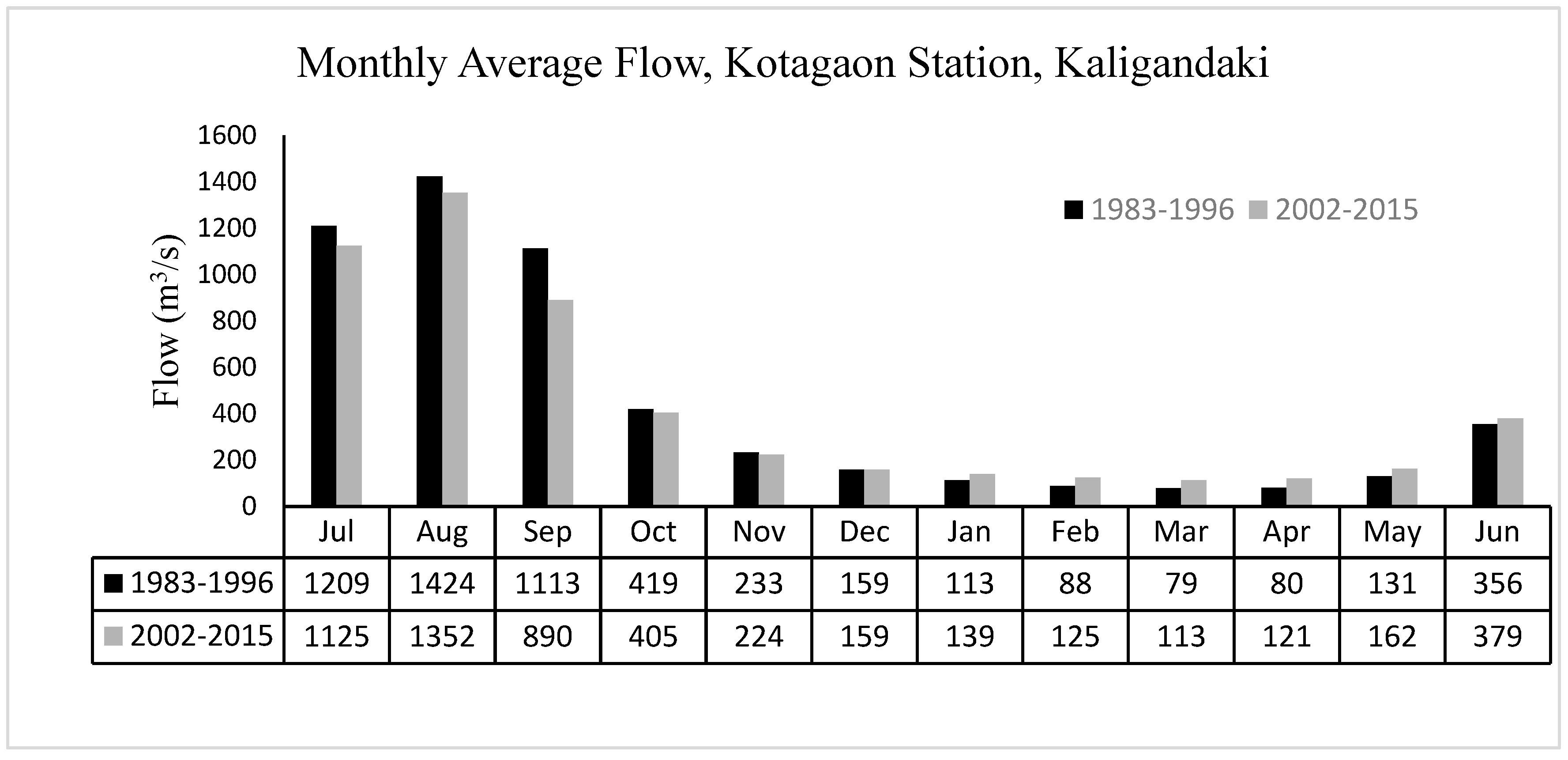
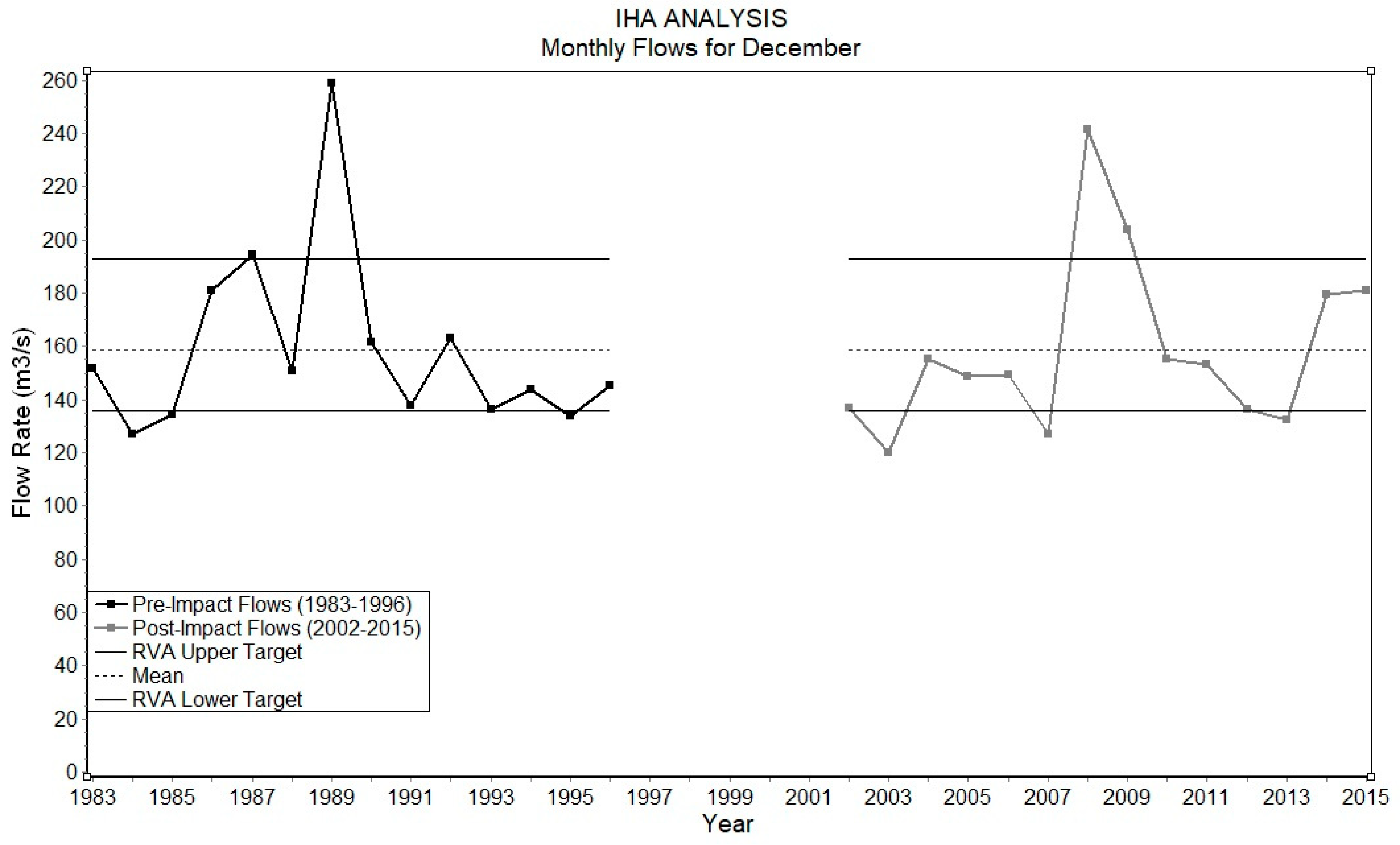
The monthly average flow comparison of January and February in Appendix A (Figure A1) suggests the change in values in the post-impact period. However, results from RVA analysis suggest zero alteration for the monthly average parameters of January and February. HCA gives non-zero alteration values for these months, potentially solving the underestimation problem of RVA. For the month of December (Figure A2), the average flow for both periods is tied up. RVA analysis also shows the equal parameters falling within the range for both periods in December. In this particular case, although RVA shows no alteration, the variation of values within the range and outside the range are not considered. The HCA method, however, gives non-zero alteration as it considers the variation within the range and outside the range too. Thus, the HCA method is established as a superior method to calculate the hydrologic alteration.

(2).

The highest value of alteration is recorded for the IHA group 5, associated with the stress on plants at floodplains and mobility of the organisms [16]. For the individual parameter, the low flow month of April shows the highest alteration value, attributed to the habitat conditions for the aquatic organisms. IHA group 2 shows the decrease in magnitude of minimum flow and increase in magnitude of maximum flow. This tends to have unfavorable habitat conditions for native species like fish. [45]. The change in timing of maximum and minimum flow associated with group 3 affects the migration and spawning of fish [46]. The change in group 4 parameters influence bed-load transport and channel sediment.

(3).

Principal component analysis reduced the 32 IHA indices/parameters of the Kaligandaki River to five parameters, namely mean monthly flow for February, mean monthly flow for March, mean monthly flow for April, mean 30-day minimum flow and mean 90-day minimum flow. These parameters are all associated with low flow values. These parameters are biologically attributed to the minimum conditions for the survival of aquatic organisms like fish [45,47,48]. These reduced parameters fully capture the hydrologic variability feature of the river in the study as explained by full 33 IHA parameters.

(4).

Combination of HCA and HYT incorporates hydrologic alteration, taking into account for both inter-year variance and intra-year variance. The combined HCA-HYT result obtained showed the hydrologic alteration in high alteration category (60.71%) for the Kaligandaki River post hydropower construction. Using the reduced IHA parameters obtained from PCA, the combined method shows moderate alteration (57.23%). The difference in results using full set parameters and reduced parameters however is only 5.72%. This highlights the effectiveness of PCA in achieving the same results through reduced parameters as compared to the full parameters of IHA. Limiting the number of parameters without affecting the explanatory feature of data helps to reduce the computational effort when used in multi-objective decision-making problems [26]. The reduced parameters can be used for future studies in the optimization of flow, considering the ecological objectives for projects like the diversion, inter-basin water transfer, hydroelectricity.

Overall, we observed the high level hydrologic alteration in the Kaligandaki River after hydropower construction. The low flow IHA parameters are affected the most. Moreover, PCA results pointed out five low flow IHA parameters as being representative hydrological indices for the basin. The peaking operation of hydropower is generally responsible for affecting the low flows [49]. This effect can be reduced by the optimal operation of hydropower, considering these low flow parameters in the ecological objective. The method explained above is suitable for less studied areas like the Kaligandaki River basin, where both cost and time are limited. Additionally, the method is less data intensive, requiring only daily flow values. The method successfully explains the alteration considering both inter-annual and intra-annual variations.

The research mentioned above calculates the flow alteration without regard to climate change. The final value of alteration is the combined effects of anthropogenic activities and climate change as a whole. Further research should be carried to separate the climate-induced alteration value from total to obtain the human-induced alteration value. Moreover, the ecological link of the representative indices should be established for detailed knowledge of ecological response to the flow changes in the river. This can provide a more robust guide for ecological flow management formulation.

References

- Sparks, R.E. Need for Ecosystem Management of Large Rivers and Their Floodplains: These phenomenally productive ecosystems produce fish and wildlife and preserve species. Bioscience 1995, 45, 168–182. [Google Scholar] [CrossRef]
- Smakhtin, V.U.; Shilpakar, R.L.; Hughes, D.A. Hydrology-based assessment of environmental flows: An example from Nepal. Hydrol. Sci. J. 2006, 51, 207–222. [Google Scholar] [CrossRef]
- Acreman, M.C.; Dunbar, M.J. Defining environmental river flow requirements? A review. Hydrol. Earth Syst. Sci. Discuss. 2004, 8, 861–876. [Google Scholar] [CrossRef]
- Poff, N.L.R. Beyond the natural flow regime? Broadening the hydro-ecological foundation to meet environmental flows challenges in a non-stationary world. Freshw. Biol. 2018, 63, 1011–1021. [Google Scholar] [CrossRef]
- Chen, W.; Olden, J.D. Evaluating transferability of flow–ecology relationships across space, time and taxonomy. Freshw. Biol. 2018, 63, 817–830. [Google Scholar] [CrossRef]
- Yu, B.; Xu, L. Review of ecological compensation in hydropower development. Renew. Sustain. Energy Rev. 2016, 55, 729–738. [Google Scholar] [CrossRef]
- Poff, N.L.; Schmidt, J.C. Managing...rivers to better meet both human and ecosystem needs is a complex societal challenge. Science 2016, 353, 1099–1100. [Google Scholar] [CrossRef]
- Tan, G.; Yi, R.; Chang, J.; Shu, C.; Yin, Z.; Han, S.; Feng, Z.; Lyu, Y. A new method for calculating ecological flow: Distribution flow method. AIP Adv. 2018, 8. [Google Scholar] [CrossRef]
- Chang, F.J.; Tsai, M.J.; Tsai, W.P.; Herricks, E.E. Assessing the ecological hydrology of natural flow conditions in Taiwan. J. Hydrol. 2008, 354, 75–89. [Google Scholar] [CrossRef]
- Tsai, W.P.; Huang, S.P.; Cheng, S.T.; Shao, K.T.; Chang, F.J. A data-mining framework for exploring the multi-relation between fish species and water quality through self-organizing map. Sci. Total Environ. 2017, 579, 474–483. [Google Scholar] [CrossRef] [PubMed]
- Richter, B.; Baumgartner, J.; Wigington, R.; Braun, D. How much water does a river need? Freshw. Biol. 1997, 047636, 231–249. [Google Scholar] [CrossRef]
- Linnansaari, T.; Monk, W.A.; Baird, D.J.; Curry, R.A. Review of approaches and methods to assess Environmental Flows across Canada and internationally. DFO Can. Sci. Advis. Secr. Res. Doc. 2012, 39, 1–74. [Google Scholar]
- Pool, T.K.; Olden, J.D. Assessing long-term fish responses and short-term solutions to flow regulation in a dryland river basin. Ecol. Freshw. Fish 2015, 24, 56–66. [Google Scholar] [CrossRef]
- Mathews, R.; Richter, B.D. Application of the Indicators of Hydrologic Alteration Software in Environmental Flow Setting. JAWRA J. Am. Water Resour. Assoc. 2007, 43, 1400–1413. [Google Scholar] [CrossRef]
- Olden, J.D.; Poff, N.L. Redundancy and the choice of hydrologic indices for characterizing streamflow regimes. River Res. Appl. 2003, 19, 101–121. [Google Scholar] [CrossRef]
- Richter, B.D.; Baumgartner, J.V.; Powell, J.; Braun, D.P. A Method for Assessing Hydrologic Alteration within Ecosystems. Conserv. Biol. 1996, 10, 1163–1174. [Google Scholar] [CrossRef]
- Poff, N.L.; Allan, J.D.; Bain, M.B.; Karr, J.R. Natural Flow Regime. Bioscience 1997, 769–784. [Google Scholar] [CrossRef]
- Acreman, M.C.; Dunbar, M.J.; Defining, M.J.D.; Acreman, M.; Dunbar, M.J. Defining environmental river flow requirements? A review. Hydrol. Earth Syst. Sci. 2004. [Google Scholar] [CrossRef]
- Arthington, A.H.; Bunn, S.E.; Poff, N.L.; Naiman, R.J. The challenge of providing environmental flow rules to sustian river ecosystems. Ecol. Appl. 2006, 16, 1311–1318. [Google Scholar] [CrossRef]
- Shiau, J.; Wu, F. Compromise programming methodology for determining instream flow under multiobjective water allocation Criteria 1. J. Am. Water Resour. Assoc. 2007, 42, 1179–1191. [Google Scholar] [CrossRef]
- Shiau, J.; Wu, F. Pareto-optimal solutions for environmental flow schemes incorporating the intra-annual and interannual variability of the natural flow regime. Water Resour. Res. 2007, 43, 1–12. [Google Scholar] [CrossRef]
- Shiau, J.; Wu, F. A histogram matching approach for assessment of flow regime alteration: Application to environmental flow. River Res. Appl. 2008, 928, 914–928. [Google Scholar] [CrossRef]
- Huang, F.; Li, F.; Zhang, N.; Chen, Q.; Qian, B.; Guo, L.; Xia, Z. A Histogram Comparison Approach for Assessing Hydrologic Regime Alteration. River Res. Appl. 2017, 33, 809–822. [Google Scholar] [CrossRef]
- Yin, X.A.; Yang, Z.F. A new method to assess the flow regime alterations in riverine ecosystems. River Res. Appl. 2015, 504, 497–504. [Google Scholar] [CrossRef]
- Li, D.; Wan, W.; Zhao, J. Optimizing environmental flow operations based on explicit quantification of IHA parameters. J. Hydrol. 2018, 563, 510–522. [Google Scholar] [CrossRef]
- Gao, Y.; Vogel, R.M.; Kroll, C.N.; Poff, N.L.; Olden, J.D. Development of representative indicators of hydrologic alteration. J. Hydrol. 2009, 374, 136–147. [Google Scholar] [CrossRef]
- Shiau, J.-T.; Wu, F.-C. Feasible Diversion and Instream Flow Release Using Range of Variability Approach. J. Water Resour. Plan. Manag. 2004. [Google Scholar] [CrossRef]
- Legendre, P.; Legendre, L. Numerical Ecology, 3rd ed.; Elsevier: Amsterdam, The Netherlands, 2003; ISBN 978-0-444-53868-0. [Google Scholar]
- Liu, Y.; Cao, S.; Yang, Y.; Zhang, X. Assessment of hydrologic regime considering the distribution of hydrologic parameters. Water Sci. Technol. Water Supply 2018, 18, 875–885. [Google Scholar] [CrossRef]
- Legendre, P.; Legendre, L. Developments in Numerical Ecology; Elsevier: Amsterdam, The Netherlands, 2013; Volume 14, ISBN 3642708803. [Google Scholar]
- Rahman, M.A.T.M.T.; Hoque, S.; Saadat, A.H.M. Selection of minimum indicators of hydrologic alteration of the Gorai river, Bangladesh using principal component analysis. Sustain. Water Resour. Manag. 2017, 3, 13–23. [Google Scholar] [CrossRef]
- Rijal, N.H.; Alfredsen, K. Environmental Flows in Nepal—An Evaluation of Current Practices and an Analysis of the Upper Trishuli-I Hydroelectric Project. Hydro Nepal J. Water Energy Environ. 2015, 17, 8–17. [Google Scholar] [CrossRef]
- Andermann, C.; Bonnet, S.; Crave, A.; Davy, P.; Longuevergne, L.; Gloaguen, R. Sediment transfer and the hydrological cycle of Himalayan rivers in Nepal. Comptes Rendus Geosci. 2012, 344, 627–635. [Google Scholar] [CrossRef]
- Mishra, B.; Babel, M.S.; Tripathi, N.K. Analysis of climatic variability and snow cover in the Kaligandaki River Basin, Himalaya, Nepal. Theor. Appl. Climatol. 2014, 116, 681–694. [Google Scholar] [CrossRef]
- Conservancy, T.N. Indicators of Hydrologic Alteration (IHA). Available online: https://www.conservationgateway.org (accessed on 12 September 2018).
- Jackson, J.E. A User’s Guide To Principal Components, 1st ed.; John Wiley & Sons, Inc.: Hoboken, NJ, USA, 1991; ISBN 0471622672. [Google Scholar]
- Abdi, H.; Williams, L.J. Principal component analysis. Wiley Interdiscip. Rev. Comput. Stat. 2010, 2, 433–459. [Google Scholar] [CrossRef]
- Arthington, A.H.; James, C.S.; Mackay, S.J.; Rolls, R.; Sternberg, D.; Barnes, A. Hydro-Ecological Relationships and Thresholds to Inform Environmental Flow Management; International Water Centre: Brisbane, Australia, 2012; ISBN 9781921499043. [Google Scholar]
- DeSarbo, W.S.; Hausman, R.E.; Kukitz, J.M. Restricted principal components analysis for marketing research. J. Model. Manag. 2007, 2, 305–328. [Google Scholar] [CrossRef]
- Kaiser, H.F. The varimax criterion for analytic rotation in factor analysis. Psychometrika 1958, 23, 187–200. [Google Scholar] [CrossRef]
- Tabachnick, B.G.; Fidell, L.S. Using Multivariate Statistics; Allyn & Bacon/Pearson Education: Boston, MA, USA, 1996; ISBN 0205459382. [Google Scholar]
- KAISER, H.F. Coefficient Alpha for a Principal Component and the Kaiser-Guttman Rule. Psychol. Rep. 1991, 68, 855–858. [Google Scholar] [CrossRef]
- Xue, L.; Zhang, H.; Yang, C.; Zhang, L.; Sun, C. Quantitative Assessment of Hydrological Alteration Caused by Irrigation Projects in the Tarim River basin, China. Sci. Rep. 2017, 7, 4291. [Google Scholar] [CrossRef] [PubMed]
- Homa, E.S.; Vogel, R.M.; Smith, M.P.; Apse, C.D.; Huber-Lee, A.; Sieber, J. An Optimization Approach for Balancing Human and Ecological Flow Needs. Impacts Glob. Clim. Chang. 2005, 1–12. [Google Scholar] [CrossRef]
- Belmar, O.; Bruno, D.; Martínez-Capel, F.; Barquín, J.; Velasco, J. Effects of flow regime alteration on fluvial habitats and riparian quality in a semiarid Mediterranean basin. Ecol. Indic. 2013, 30, 52–64. [Google Scholar] [CrossRef]
- Gao, B.; Li, J.; Wang, X. Analyzing changes in the flow regime of the Yangtze River using the eco-flow metrics and IHA metrics. Water (Switzerland) 2018, 10, 1552. [Google Scholar] [CrossRef]
- Phelan, J.; Cuffney, T.; Patterson, L.; Eddy, M.; Dykes, R.; Pearsall, S.; Goudreau, C.; Mead, J.; Tarver, F. Fish and Invertebrate Flow-Biology Relationships to Support the Determination of Ecological Flows for North Carolina. J. Am. Water Resour. Assoc. 2017, 53, 42–55. [Google Scholar] [CrossRef]
- Sinnathamby, S.; Douglas-Mankin, K.R.; Muche, M.E.; Hutchinson, S.L.; Anandhi, A. Ecohydrological index, native fish, and climate trends and relationships in the Kansas River basin. Ecohydrology 2018, 11. [Google Scholar] [CrossRef] [PubMed]
- Räsänen, T.A.; Someth, P.; Lauri, H.; Koponen, J.; Sarkkula, J.; Kummu, M. Observed river discharge changes due to hydropower operations in the Upper Mekong Basin. J. Hydrol. 2017, 545, 28–41. [Google Scholar] [CrossRef]
Figure 1.
The study area, Kaligandaki River basin.
Figure 2.
Schematic layout of the calculation methodology.
Figure 3.
Scree Plot of Eigenvalues and Cumulative Variances (Pearson Method).
Figure 4.
Scree Plot of Eigenvalues and Cumulative Variances (Spearman’s Method).