Article

Hydrodynamic Characterization of Sustainable Urban Drainage Systems (SuDS) by Using Beerkan Infiltration Experiments

by
Sofia Bouarafa
1,2,*,
Laurent Lassabatere
1,
Gislain Lipeme-Kouyi
2 and
Rafael Angulo-Jaramillo
1
1
UMR5023 Ecologie des Hydrosystèmes Naturels et Anthropisés, Université de Lyon, 3 rue Maurice Audin, 69518 Vaulx-en-Velin, France
2
Laboratory of Wastes Waters Environment and Pollutions (DEEP), University of Lyon, INSA Lyon, 69621 Villeurbanne, France
*
Author to whom correspondence should be addressed.
Water 2019, 11(4), 660; https://doi.org/10.3390/w11040660
Submission received: 8 February 2019 / Revised: 27 March 2019 / Accepted: 27 March 2019 / Published: 30 March 2019
(This article belongs to the Special Issue Soil Hydrology for a Sustainable Land Management: Theory and Practice)

Abstract

:
Stormwater management techniques in urban areas, such as sustainable urban drainage systems (SuDS), are designed to manage rainwater through an infiltration process. In order to determine the infiltration capacities of different SuDS and to identify their unsaturated hydraulic properties, measurements with the Beerkan method (i.e., single ring infiltration tests) were carried out on four types of common infiltration structures in an urban zone of Lyon (France): A drainage ditch with an underlying storage structure, a parking lot with a waterproof pavement that transfers runoff water toward the ditch, a vegetated hollow core slab, and an embankment of a grass-covered garden that was used as a reference for rainwater infiltration capacity. The novelty of this study lies in the use of three Beerkan estimation of soil transfer parameters (BEST) algorithms: BEST-slope, BEST-intercept, and BEST-steady to analyze infiltration data. The BEST methods are based on the analysis of the infiltration rate from transient to steady-state flow. They allow the determination of both shape and scale parameters of the soil water retention curve h(θ) and the hydraulic conductivity curve K(θ). The three BEST methods are efficient and simple for hydraulic characterization of SuDS. The study of the hydrodynamic behavior of the four structures revealed the infiltration inefficiency of some of them. Their average infiltration rates are considerably lower than the reference infiltration rain garden. The results confirmed the impact of some physical conditions, such as pore structure modification due to invasive vegetation colonization and the presence of soil organic matter, on soil hydrodynamic behavior degradation.

1. Introduction

The guidelines for urban stormwater management have undergone several changes over the course of time. They were based first on hydraulic and hygienist premises, which consist of quick evacuation of stormwater toward natural aquatic environments through separate or combined sewer systems. These conventional drainage systems only consider water quantity management issues, and they are economically and ecologically costly. Growth of waterproofed surfaces, as well as climate change, has generated an important rise in flood events in urban areas because of the limited capacity of sewage networks. Diverse activities pursued in cities produce a large variety of pollutants that are disposed in air and on surfaces. They can be organic, such as hydrocarbons, oils, and grease; inorganic, such as metals and dissolved nutrients; or pathogenic microorganisms, such as bacteria and viruses [1,2,3]. All of these contaminants end up in the receiving water bodies [4,5,6].
Currently, stormwater management in urban areas embodies a qualitative approach that consists of restoring rainwater into a hydrological cycle that has to be close to the natural process, by limiting runoff and fast water accumulation. New techniques have been innovated to fulfill the double criteria of quantitative and qualitative water management. They are commonly called SuDS: Sustainable urban drainage systems [7].
SuDS are designed to substitute and/or supplement pipe network systems. They are based on decentralization of the stormwater treatment point, i.e., stormwater is managed close to its drop point through an infiltration process. There are several types of SuDS: e.g., infiltration basins, ditches, rain gardens, and porous pavements. Their hydraulic efficiency relies on two main standards that are infiltration and retention capacity [8,9,10]. Globally, the infiltration capacity should be high enough to prevent flooding while enabling pollution removal processes through settling and adsorption.
The infiltration capacity of a soil is usually estimated by measuring the rate at which water soaks away from test pits or boreholes [11,12]. However, further information about the hydrodynamic characteristics of the soil would be helpful to assimilate water transfer profiles. Depending on their texture, porosity, particle size distribution, and hydric history, some soils will provide better contaminant retention, while others are more likely to develop preferential pathways promoting direct transfer of contaminated water toward the underground water table [13,14,15].
Attention will be devoted in this paper to the assessment of SuDS infiltration capacity through the determination and analysis of their hydrodynamic characteristics by using the Beerkan estimation of soil transfer parameters (BEST) method, which is an effective well-tried method in the field of hydrodynamic property characterization of different soil textures [16,17,18]. The BEST method relies on the analysis of in situ infiltration data built by the Beerkan infiltration protocol. The Beerkan infiltration method was introduced by Haverkamp et al. (1996) [19]. It is a simple, inexpensive, and repeatable method that quantifies water infiltration curves in porous media. It consists of infiltrating known water volumes under saturated conditions through a ring, until reaching steady-state infiltration. By exploiting the resulting infiltration curve, bulk density, particle size distribution, and hydric conditions, the BEST method provides an estimation of saturated hydraulic conductivity Ks, sorptivity S, and shape and scale parameters of soil–water relationships.
The BEST method outputs allow the determination of hydraulic conductivity K(θ) and hydraulic retention curves h(θ) by Equation (1) of van Genuchten et al. (1980) [20] under the Burdine condition [21], Equation (2), and Equation (3) of Brooks and Corey [22], respectively.
( θ θ r ) ( θ s θ r ) = [ 1 + ( h h g ) n ] m
m = 1 2 n
K ( θ ) = K s ( θ θ r θ s θ r ) η
where θr and θs (L3 L−3) are the residual and saturated volumetric water contents, respectively. θr is assumed to be zero. Ks (L T−1) is the saturated hydraulic conductivity; n, m, and η are the shape parameters; and hg is the pressure head scale parameter of h(θ) calculated from the sorptivity, as follows:
S 2 ( θ 0 , θ s ) = c p θ s K s h g ( 1 θ 0 θ s ) [ 1 ( θ 0 θ s ) η ]
where θ0 is the initial volumetric water content and cp is a constant derived by Haverkamp et al. (1999) [23]:
c p = Γ ( 1 + 1 n ) [ Γ ( m η     1 / n ) Γ ( m η ) + Γ ( m η   +   m     1 / n ) Γ ( m η   +   m ) ]
where Γ is the incomplete gamma function.
There are three different BEST methods to estimate parameters Ks and S: BEST-slope [18], BEST-intercept [24] and BEST-steady [25]. They differ according to the fitting method of infiltration equations to experimental data.
By using the parameters Ks and S obtained by the three BEST methods, the macroscopic capillary length scale λc (L) and the average characteristic size of hydraulically activated pores λm (L) can be calculated by using the equations of White and Sully (1987) [26] and Warrick and Broadbridge (1992) [27]:
λ c = b S 2 ( θ f θ i ) K s
λ m = σ ρ w g   1 λ c
where b is a constant depending on soil water diffusivity function, and it is frequently considered that b = 0.55. θi and θf are the initial and final volumetric water contents, respectively. σ is the surface tension of water (σ = 73 mN m−1), ρw is water density, and g is the acceleration due to gravity.
The BEST methods have been successfully used to characterize different soils with different textures. Lassabatere et al. (2006) [18] applied the method on three different types of soils: An agricultural soil, a sandy soil, and a fluvioglacial deposit. Acceptable estimations of the hydraulic parameters were provided for the three soils. Yilmaz et al. (2010) [24] used the BEST method to define unsaturated hydraulic properties of a Basic Oxygen Furnace (BOF) slag in order to study the impact of spatial heterogeneity and follow its evolution through time. Bagarello et al. (2012) [28] used the BEST method to estimate the soil water retention curve of 199 Sicilian soils and discussed the efficiency of the method by comparing the results to reference soils from a known database. The study concluded that BEST water retention model can be appropriate for most soils. Di Prima et al. (2015) [17] used a Beerkan automatic device combined with the BEST algorithms to study the hydraulic properties of three agriculture soils. The results showed that the BEST methods can be a good substitute to laboratory measurements to define the hydraulic properties of soils.
In this study, the BEST methods were applied to four current urban stormwater management structures located in Lyon (France) in order to evaluate their infiltration capacity and identify possible malfunctioning through the study of their hydrodynamic parameters and curves. The studied structures include: (i) A drainage ditch with an underlying storage structure, (ii) a parking lot with a waterproof pavement that transfers runoff water toward a ditch, (iii) a vegetated hollow core slab, and (iv) an embankment of a grass-covered garden that was used as a reference for rainwater infiltration capacity. The observations and conclusions related to these structures cannot be generalized. The hydrodynamic functioning of each SuDS depends on multiple intrinsic conditions such as PSD, water content, vegetation cover, etc. Similar functioning cannot be expected for two SuDS of the same design. The main objective of this paper is to evaluate the convenience of using the BEST methods to determine the characteristic hydrodynamic parameters of SuDS in order to monitor their efficiency. The impact of erosion and some other physical conditions influencing the infiltration capacity of SuDS are discussed through the obtained results. A comparison of the outcomes of the three BEST methods was performed by a statistical analysis.

2. Materials and Methods

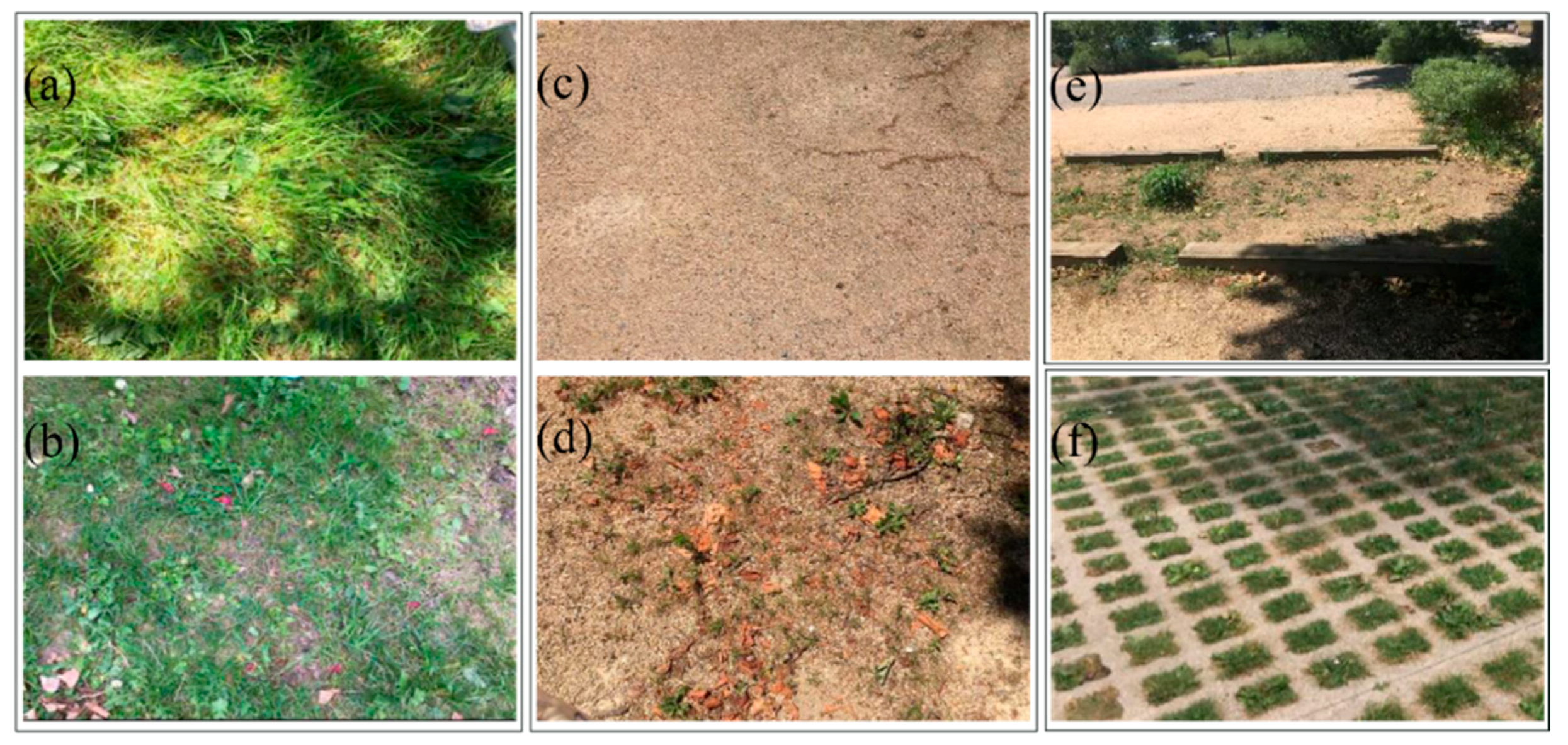
2.1. Studied Sites and Structures

The city of Lyon experiences significant rainfall events. The average annual precipitation height is around 831.9 mm, corresponding to 104.1 rainy days (1981–2010). The studied stormwater management structures were located in the east of Lyon in Lyon university campus, which is a pilot site for urban green city renovation as part of the Lyon city Field Observatory for Urban Water Management (OTHU). The studied structures were a reference grass-covered embankment, an impervious parking lot, a drainage ditch, and a vegetated hollow core slab. They receive the same type of runoff, mainly originating from parking lots, sidewalks, and circulation lanes.
The reference structure was a grass-covered garden embankment that had no specific infiltration or storage design (Figure 1a,b). Urban surfaces of this kind (gardens, parks, etc.) play an important role in ensuring rainwater infiltration. This structure was considered as a reference because it is the closest to natural soil. Infiltration tests were conducted in two different areas of this embankment, located within a dozen meters. They were called “Embk 1” and “Embk 2”.
The first stormwater management structure was a parking lot incorporating a waterproof pavement (Figure 1c). This structure is not an infiltration system. The parking lot surface is only expected to grant water runoff to a nearby receiving ditch. After four years of use, some parts of the parking lot surface were subject to alterations and cracks because of invasive plant colonization (Figure 1d). In this study, it was referred to as “PKG-Int” and “PKG-Alt” for the intact and the altered areas, respectively. Both areas were studied separately to acknowledge the impact of invasive vegetation and surface deterioration on impervious surfaces.
The second structure was the drainage ditch, also called a dry swale, that receives the nearby waterproof parking lot runoff (Figure 1e). It is an experimental structure that receives stormwater from a 302.3 m² catchment area. The bottom of this structure is waterproofed. Rainwater infiltrates through 300–600 mm of topsoil, then through a filtration geotextile membrane, before reaching a calibrated gravel layer connected to a 160 mm diameter draining pipe. The drain outlet effluents are gathered in an underground storage structure where water quality is monitored. This structure was referred to as “the Ditch.”
The last studied structure was the vegetated hollow core slab, also called a concrete grid parking lot (Figure 1f). It is a grass–concrete reinforced structure that is able to support significant loads (the weight of cars, passage of pedestrians, etc.) and infiltrate rainwater and runoff through topsoil-filled cells. The structure underneath the topsoil is permeable and includes a geotextile filtration layer. The depth of topsoil in the cells is well conceived to ensure that the soil will not be compacted through usage. It was referred to as “Grid-PKG”.

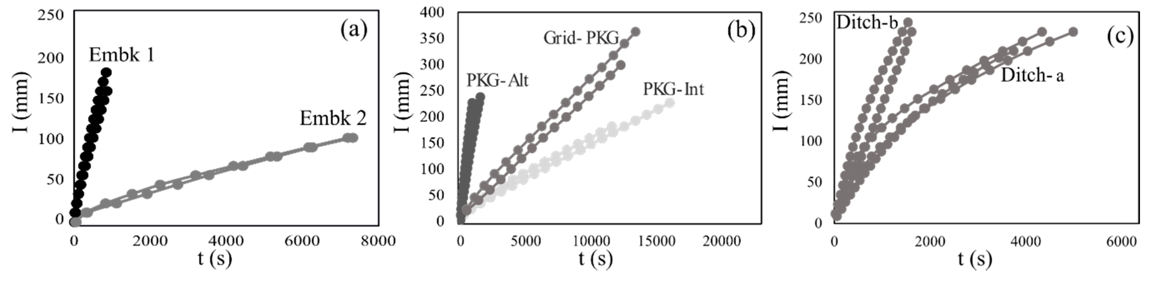
2.2. Infiltration Tests

Before starting a Beerkan test, the ground surface must be prepared. If the studied area is vegetated, plants must be cut while keeping the roots in situ. A ring is then positioned on the surface and embedded carefully, without destroying the soil’s structure, to a depth of less than 1 cm in order to avoid lateral water losses. Bentonite can be used to secure the outer edges of the ring, especially in the case of coarse-textured soils. Constant water volumes are infiltrated successively through the ring under a surface-saturated condition, and the time needed for the entire infiltration of each volume is recorded. The test is stopped once the infiltration time is stabilized, i.e., when at least three consecutive infiltration times are identical [29]. In general, a set of 8–15 water volumes will achieve steady-state infiltration [18]. A sample is quickly collected at the end of the test from the ring center to determine the final volumetric water content. An undisturbed core is collected nearby the test spot to determine both soil bulk density and initial volumetric water content. Another soil sample is collected to determine the particle size distribution (PSD).
Beerkan tests were carried out on five different spots of Embk 1, two spots of Embk 2, seven spots of PKG-Int, six spots of PKG-Alt, seven spots along the Ditch, and eight cells of Grid-PKG. Infiltration rings of 15 cm diameter were used for all the tests, except for Grid-PKG for which 7.5 cm diameter rings were used so as to fit the cells’ dimensions. 100 mL volumes of water were used for infiltrating.
To define the particle size distribution of each soil, the collected samples were oven dried before being manually sieved to a 1.3 mm particle size. Thereafter, a fine proportion of the soil matrix was analyzed by a laser particle size analyzer (Mastersizer 2000, Malvern, UK).

2.3. BEST Method for Hydraulic Parameter Estimation

The BEST method was developed to estimate hydraulic parameters Ks and S, as well as shape parameters n, m, and η, and to define the water retention curve h(θ) and the hydraulic conductivity curve K(θ), determined by Equations (1) and (3), respectively.
The scale parameter Dg and shape parameters M and N are estimated by fitting the cumulative frequency F(D) (Equations (8) and (9) in Table 1) to the particle size distribution of the soil’s fine fraction (<2 mm). The estimation of the soil fractal dimension (Equations (10) and (11) in Table 1) then allows the computation of the shape index parameter pm (Equation (12) in Table 1) and subsequently the shape parameters n, m, and η directly by solving Equations (12)–(16) in Table 1.
The hydrodynamic parameters Ks and S are estimated by fitting experimental infiltration data to the analytical axisymmetric infiltration model of Haverkamp et al. (1994) [32] (Equations (17)–(21) in Table 2). They can be calculated by the three BEST methods: Slope, intercept, and steady. The three methods define Ks and S by making different use of the parameters iexp and bexp, which are both estimated by a linear regression analysis of the data that describes the steady-state condition of the cumulative infiltration curve I(t). BEST-slope and BEST-intercept are based on the model of Haverkamp et al. (1994) [32] that fits transient-state experimental data to estimate sorptivity S and then the saturated hydraulic conductivity Ks. BEST-slope uses the slope iexp (Equations (22) and (23) in Table 2), and BEST-intercept uses the intercept bexp (Equations (24) and (25) in Table 2), whereas BEST-steady uses both parameters and does not require additional experimental data fitting (Equations (26) and (27) in Table 2).

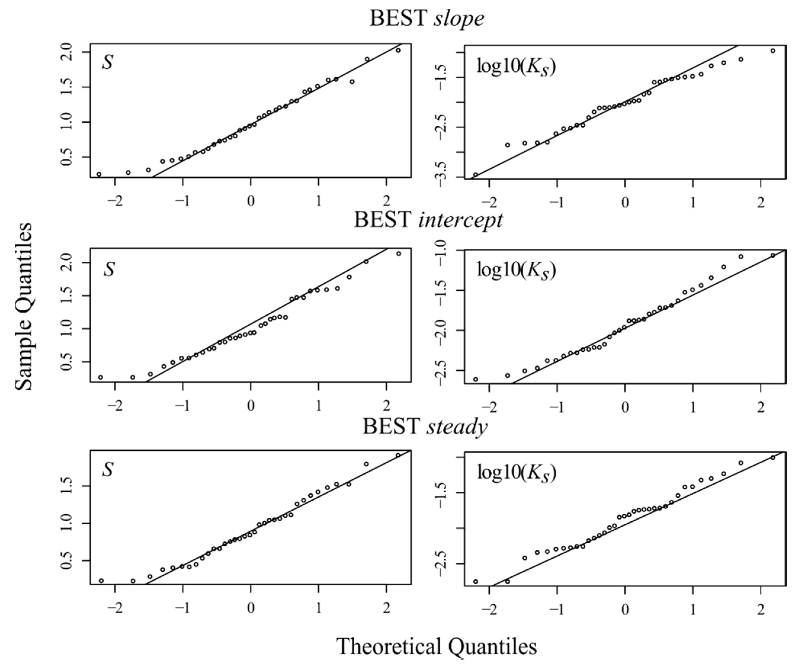
2.4. Statistical Analysis

Estimates of Ks and S by the three BEST methods were statistically analyzed. In order to evaluate the influence of the studied structure on the variance of parameters Ks and S, one-way ANOVA tests were performed. These tests can be used to determine any statistical significance between variables by calculating two main parameters: The F-value, which is the ratio of the variation between sample means to the variation within the sample, and Pr(>F), which represents the non-significance hypothesis probability. Pr(>F) should be compared to a critical significance level, usually 5%, in order to assess the non-significance of the hypothesis.
Normal/log-normal distribution verifications of both parameters Ks and S were elaborated by using the Quantile-Quantile (QQ) plots and the Kolmogorov–Smirnov tests (R core team, 2013). QQ plots represent the quantiles of experimental data against theoretical probability distribution quantiles, in our case, the normal or log-normal distribution. The distribution is considered to be normally or log-normally distributed if the points in the QQ plot are arranged close to the first bisector y = x. The Kolmogorov–Smirnov (K-S) test quantifies the distance between the reference distribution and the studied sample distribution. This test calculates the parameter D-value that represents the maximal distance between the two distributions and the parameter p-value that refers to the probability of observing a higher distance than the D-value. The p-value should be compared to a critical statistics threshold in order to decide if the sample is normally or log-normally distributed. Usually, 5% is used.
For each test, the estimations of parameters Ks and S were plotted as a function of the average of the BEST-slope, intercept, and steady estimates in order to compare the three methods. Linear regression models were then used to test the correlation between Ks and S and assimilate soil capillary and gravity drainage functioning.
BEST graphs and estimations were elaborated by using the open-source software Scilab, while R was used for the statistical analysis (R Core Team, 2013). Box-and-whisker plots were used to represent the estimates of Ks, S, and λm. They are able to depict each structure’s statistic values: The median, the upper, and lower quartiles and the highest and lowest values. This representation can be used to compare the studied structures and assimilate variability within the same structure.

3. Results and Discussion

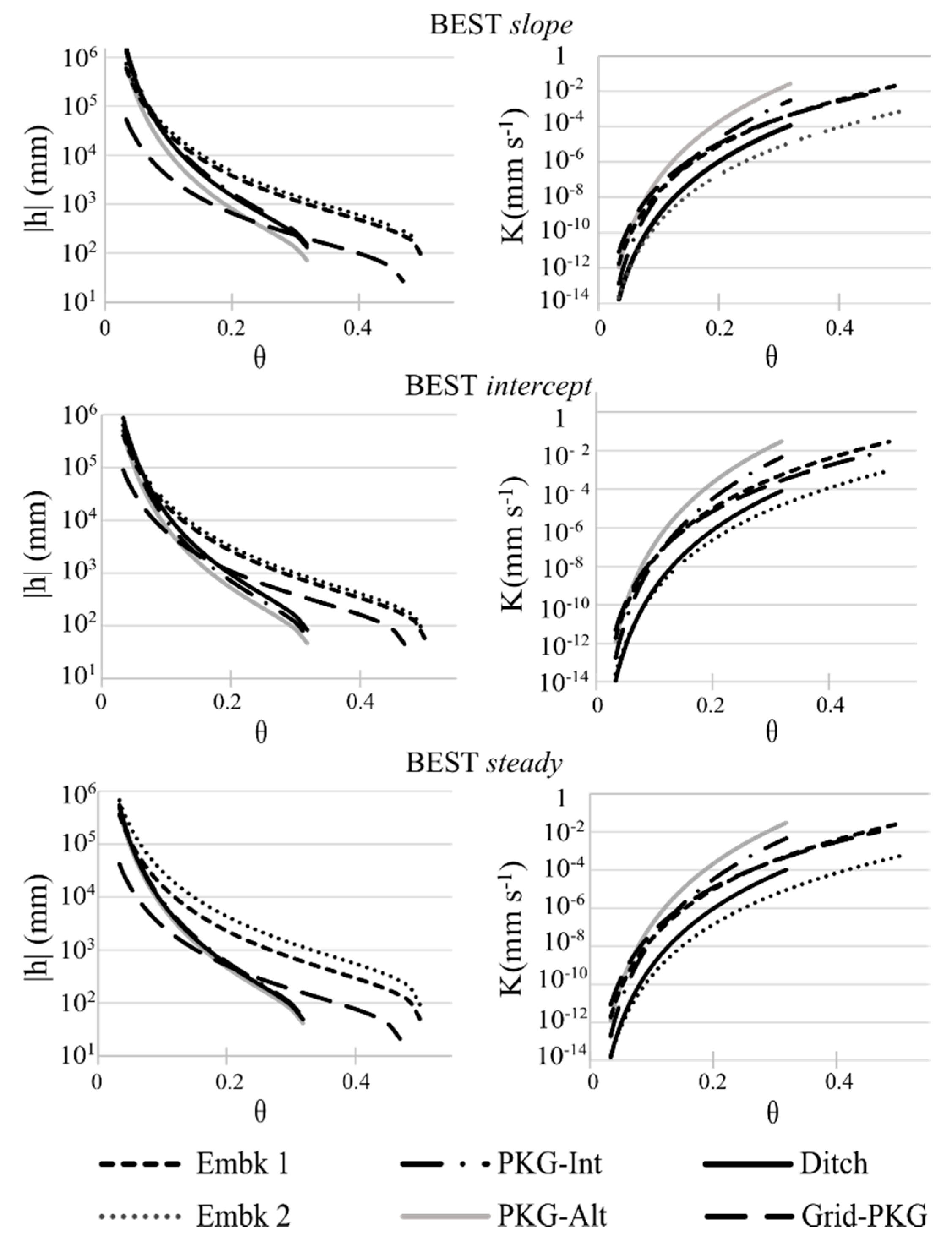
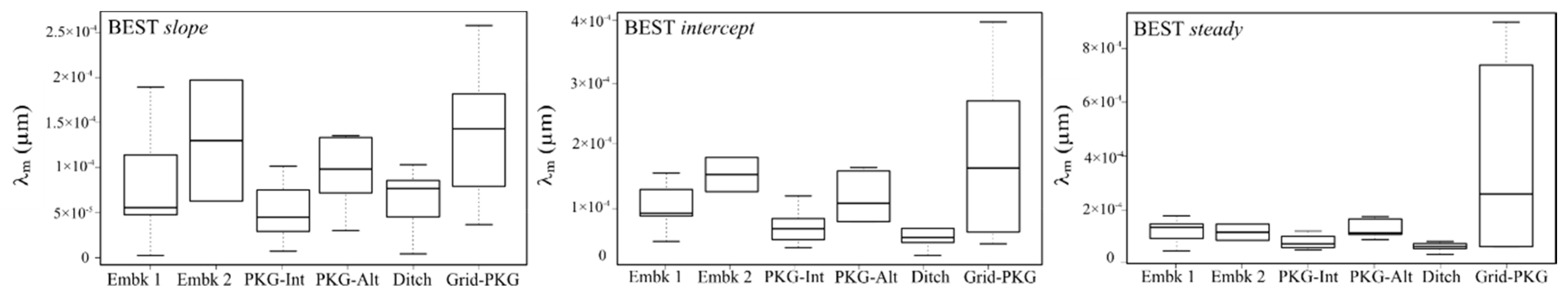
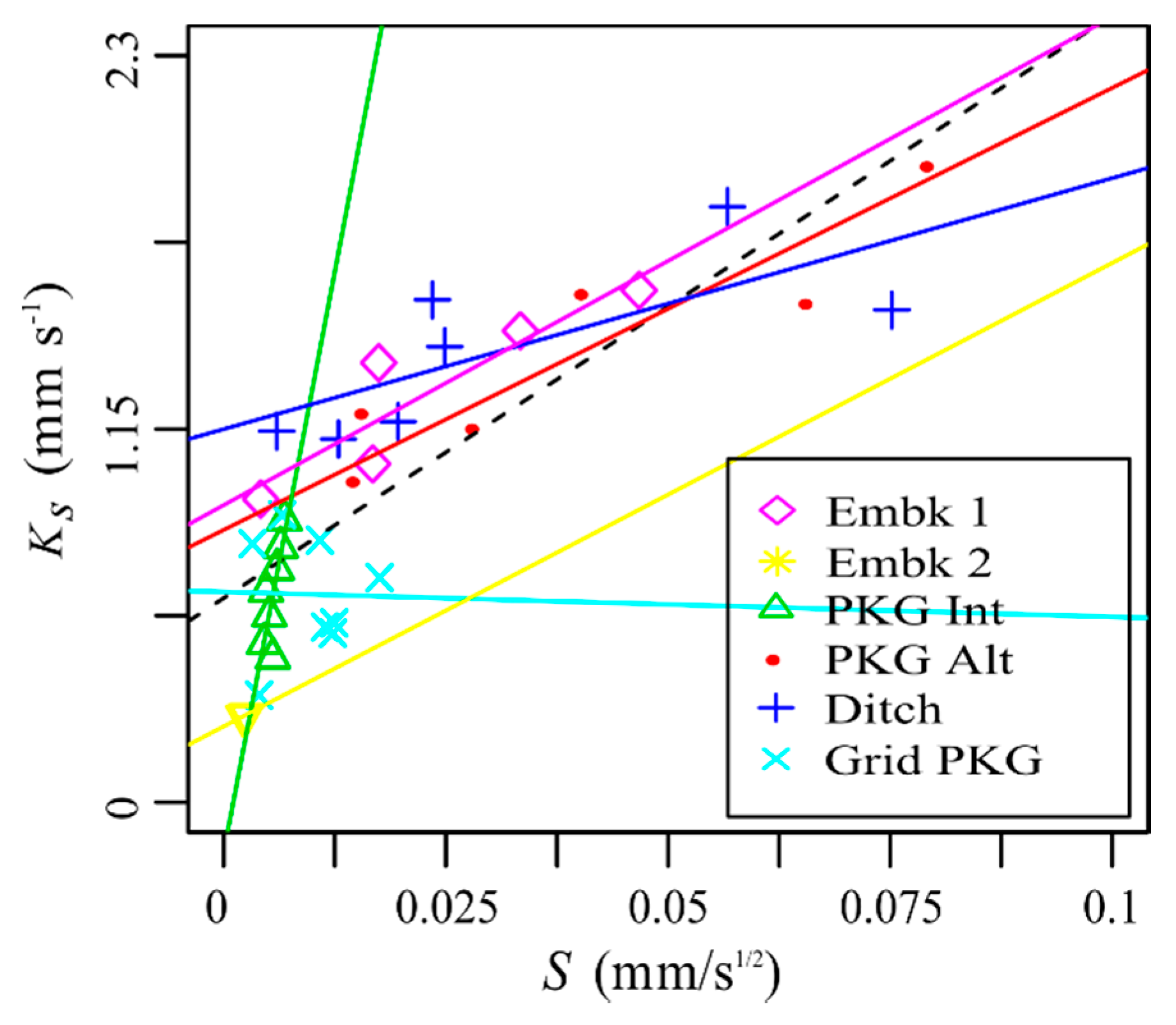
3.1. Hydrodynamic Characteristics of SuDS

All soils have mainly a silty-sandy texture (Figure 2a,b). Particle size distributions of the fine fractions (<1.3 mm) revealed the bi-modality of the waterproof parking lot and the Ditch. The proportion of coarser particles (>1.3 mm) varied between 5% (Embk 2) and 66% (waterproof parking lot, PKG-Int, or PKG-Alt) of the sample’s total weight.
Shape parameters n, m, η, and cp were defined from fine fraction PSD fitting (Figure 2c). The waterproof parking lot and the Ditch had similar shape parameter values, slightly lower than the other soils (Table 3). Grid-PKG and both the studied embankments had close values.
Examples of experimental Beerkan cumulative infiltration curves of each structure are presented in Figure 3. The conducted tests on both areas of the reference garden embankment showed a significant infiltration flow in Embk 1 (infiltration rate ≈ 10−1 mm s−1), whereas a low infiltration rate was recorded in Embk 2 (infiltration rate ≈ 10−2 mm s−1). This finding can be explained by the narrow particle size distribution of Embk 2 and its low proportion of coarse particles (>1.3 mm). Apart from the potential presence of biological pores, such as earthworm channels, macropores were accordingly almost inexistent in this structure. Besides, a comparison of the initial and final water contents indicated that θfinal ≈ 1.5 θinitial, which suggests that the soil was initially very wet. Microporosity, which was the overriding porosity in this structure, must have been nearly saturated from the beginning of infiltration. This observation also explains the absence of an infiltration transient state on the infiltration curves (Figure 3a). These conditions are susceptible to lead later to erroneous estimations of the hydraulic parameters by the BEST methods.
The Beerkan infiltration curves revealed a big difference in infiltration capacity between PKG-Int and PKG-Alt. The flow at the level of the altered area was approximately four times greater than that of the intact area (Figure 3b). This was due to the presence of cracks and macropores created by plant roots. It is important to note that the mean infiltration rate of PKG-Int was 2.2 × 10⁻² mm s−1. This is greater than 10−5 mm s−1, which is the reference value to qualify a soil as pervious [34]. These results show that the surface coating of this parking lot was inefficient in both altered and intact areas because of a design failure and erodible material choice.
Infiltration curves of the drainage ditch revealed infiltration rates in the order of 9 × 10⁻² mm s−1 (Ditch-a in Figure 3c). The marked concavity at the first moments of infiltration reflected the importance of capillary forces (i.e., significant sorptivity). At some spots for this structure, the infiltration curves showed a sudden increase after a certain infiltration time (Ditch-b in Figure 3c). This was probably related to the presence of swelling organic matter in the soil creating a capillary barrier effect [16,35], which favored evolution of preferential pathways around the organic matter zones. It might also have resulted from pore clogging induced by siltation in some areas. Structures with infiltration rates greater than 10−2 mm s−1 are potentially exposed to this phenomenon [9]. The risk of pore clogging was more important in the Ditch since the nearby parking lot ensured that the runoff held a high proportion of silt and was, above all, subject to erosion. Another interpretation is possible regarding the consistence of the pollutants the Ditch was susceptible to receive. In fact, the parking lot surface could potentially have been covered by greasy car emissions. These hydrophobic pollutants were carried by rainwater and end up on the Ditch surface, leading in the same way as organic matter to a barrier effect [16].
In Grid-PKG, the mean infiltration rate was 3.4 × 10⁻² mm s−1. This low infiltration capacity was probably due to clogging [36,37,38] or hydrophobicity effects. The extremely low initial volumetric water content in this structure (θfinal = 13 θinitial) may have led to water repellency at the beginning of the infiltration tests. Water repellency can be expected when soil water content is below a threshold value [39]. This case illustrates the importance of water content history knowledge to predict the hydrodynamic behavior of a soil. Vegetation was also dense in the Grid-PKG cells. Biofilms on plant roots may have been the origin of this hydrophobic behavior [40,41].
The fitting of Haverkamp’s equations (Equations (17) and (18) in Table 2) [32] on Beerkan curves could be used to estimate S and Ks by the three BEST methods; this is shown in Figure 4. Embk 1 had significant values of Ks and S. Its saturated hydraulic conductivity was significant due to the wide particle size distribution favoring the presence of macropores and, thus, gravity flow [42,43,44]. At the same time, the presence of a large proportion of fine materials (silt) led to significant sorptivity values [45]. The lowest values of Ks and S were obtained by Embk 2 as a consequence of its narrow particle size and low proportion of fine particles.
PKG-Alt had the highest values of Ks and S (Figure 4). Its saturated hydraulic conductivity was significant due to the presence of cracks created by plants roots favoring gravity flow. This structure was also composed of a high proportion of fine materials (silt and clay), leading to significant sorptivity values. The parking lot area had the largest variation range of both parameters Ks and S because of the soil heterogeneity, regarding vegetation density and erosion extent. Lower values of saturated hydraulic conductivity and sorptivity were observed for PKG-Int.
Estimates of Ks and S for Ditch were in approximately the same order as the reference structure Embk 1, unlike Grid-PKG that had lower values. This result was in agreement with its low infiltration rates.
By considering the average values of saturated hydraulic conductivity and sorptivity for each BEST method, characteristic curves h(θ) and K(θ) were established by using Equation (1) of van Genuchten [20] and Equation (3) of Brooks and Corey [22] (Figure 5). The three BEST methods gave similar results. Water retention curves of PKG-Int, PKG-Alt, and the Ditch had a sudden variation with θ, represented by a steeper slope. Their hydraulic conductivity curves also evolved with θ quicker than the other structures. This resulted from their high proportion of coarse particles and their bimodal particle size distribution (Figure 2a,b). This proportion of coarse material presented a wide range of macropores that were the first to be hydraulically activated at the beginning of infiltration at high pressure and accordingly had higher saturated hydraulic conductivities [18] (Figure 5). This explains the rapid response of h(θ) and K(θ). Moreover, because of their bimodal PDS, once the water pressure reached the activation value of the average size pores corresponding to the first distribution mode, most of the pores became saturated. Consequently, h(θ) and K(θ) varied steeply with θ [18].
For the other structures, the water retention curves had smoother slopes with a plateau because of their fine and extended particle size distribution. Their pores were gradually saturated, which explains the slower variation of K(θ) and h(θ).
Parameter λm, the mean characteristic radius of hydraulically activated pores, was calculated for each structure after Equation (7) by using hydraulic conductivity, Ks, and sorptivity, S, estimates by the three BEST methods. The mean pore radii of the studied structures varied in the intervals [18–260 μm] by BEST-slope, [39–390 μm] by BEST-intercept, and [0.05–890 μm] by BEST-steady (Figure 6).
Apart from Grid-PKG and Embk 2, the three BEST methods gave proximate results for the rest of the studied structures. The obtained values also matched their corresponding observed mean infiltration rates (Table 4). Structures with high mean hydraulically activated pore radii were most likely to have a significant infiltration flow and vice versa. The largest differences between the three methods and the least coherent results were noticed in Grid-PKG and Embk 2. The calculated mean radii of these two structures were very significant and did not correspond to their slow infiltration flows. Their special hydric initial conditions explain the erroneous estimates for Ks and S. For Embk 2, the soil was initially very wet, a steady state was quickly reached, and thus, the transient state was poorly described. This implies an incorrect estimation of sorptivity, especially in the cases of BEST-slope and BEST-intercept, which rely on transient-state data fitting. For Grid-PKG, soil water repellency made steady-state infiltration hardly reachable. Hence, too few data points were collected, which confused the BEST-slope and intercept results [16,17]. Parameter Ks was then overestimated, and S was under-estimated [46], which explains the overestimation of λm.
Accordingly, it is important to make sure that while conducting a Beerkan infiltration test a steady state is reached, and the soil is initially dry enough to acquire transient-state describing data. In general, it must meet the condition θinitial < 0.25 θsaturated [32], without being overly dry to avoid water repellency problems [39].

3.2. Statistical Analysis of the Three BEST Methods

A comparison between Ks and S values, as well as the characteristic curves K(θ) and h(θ) obtained by the three BEST methods, shows globally coherent results. This outcome was confirmed by the correlation coefficients. A considerable correlation between BEST-slope and BEST-steady was observed in terms of both parameters Ks and S (coeff(Ks) = 0.93 and coeff(S) = 0.99). A slightly weaker correlation was noticed between BEST-slope and BEST-intercept for the parameter Ks (coeff(Ks) = 0.60). BEST-slope failed to properly calculate Ks and S in some cases (4 tests out of 43). This was probably due to the lack of precision when choosing steady-state points, especially in low permeability soils where steady-state could hardly be achieved. It could also result from the soil’s initial hydric conditions that could distort the description of the transient state [16,17]. The first infiltration moments are the moments when capillary forces are predominant. When initial water content was high, the infiltration curve did not represent the sorptivity impact which influenced the calculations of both S and Ks.
One-way ANOVA tests on parameters Ks, S, and the average infiltration rate (IR) allowed F-values and Pr(>F) to be calculated. For Ks, F-value = 4.325 and Pr(>F) = 0.00462. For S, F-value = 16.4 and Pr(>F) = 1.09 × 10⁻⁷. For IR, F-value = 7.284 and Pr(>F) = 1.59 × 10⁻⁴. These results suggest that the variability of Ks, S, and IR of the different structures (with a threshold of significance of 5%) was significant compared to the variability within the same structure.
The normality tests showed that sorptivity, S, is normally distributed, while saturated hydraulic conductivity is log-normally distributed, as shown in the QQ plots (Figure 7). This result was confirmed by the Kolmogorov–Smirnov tests, for which we considered a threshold value of 5% (Table 5). Similar observations were made as part of other studies of the BEST methods [17].
For each test, Ks was represented as a function of the geometric average of the estimations by the three BEST methods (Ks being log-normally distributed), and S was represented as a function of the arithmetic average (S being normally distributed) (Figure 8). The three methods gave results ranging around the mean with a slight underestimation of the sorptivity by BEST-slope and a minor overestimation of the same parameter by BEST-steady. Therefore, use of the geometric average of Ks and the arithmetic average of S to plot Ks vs. S can be justified.
The obtained Ks vs. S plot defines a point cloud with a positive slope tendency (dashed line in Figure 9). This plot displays two groups of soils. The first group contained tests with low values and low variance of both parameters Ks and S. They belonged mainly to Embk 2, PKG-Int, and Grid-PKG. These structures had a low infiltration capacity due to their initial hydric condition and/or their homogenous particle size distribution. The second group contained the rest of the structures that had significant and diffuse values of Ks and S due to their heterogeneous textures and structures: Extended PSD, large fraction of fine particles, presence of macropores, cracks, vegetation, etc.
This representation of Ks vs. S enables the infiltration flow to be indexed, in a general way, as predominantly sorptive or gravity driven. For SuDS, this information can be crucial to pertinently choosing conception materials that allow both good infiltration and retention capacity. Soils with high values of Ks and S would be the best options to ensure good functioning. Following the evolution of the point cloud of a SuDS through time with this representation could also be interesting, in order to identify the origin of a possible malfunction.

4. Conclusions

The three BEST methods gave globally similar results and enabled the most important hydrodynamic parameters of the studied SuDS to be successfully determined. However, under extreme water content conditions, either initially very dry or very wet soils, the obtained results of the three methods were less accurate.
SuDS are accumulation points of rainwater, which makes of them a source of possible contaminant transfer toward the water table. The application of the BEST method allowed to evaluate the risk of dysfunctioning, related to their infiltration capacity or contaminant retention, through the study of hydrodynamic parameters Ks and S, water retention curve h(θ), and hydraulic conductivity curve K(θ). It also allowed the representation of soils in terms of their sorptivity/gravity infiltration capacity, in order to identify malfunctioning SuDS.
This study showed that continuous monitoring of SuDS infiltration capacity is essential, especially when structures are subject to erosion, as was the case of the studied waterproof parking lot that turned out to be permeable because of a design defect. The invasive vegetation in the altered areas led to high infiltration flows. This means that a significant proportion of the parking lot runoff was infiltrated before reaching the ditch, which presents an important hazard of contaminants (e.g., automobile emissions) being transferred to the underlying groundwater. The increase of the infiltration flow in the altered areas by invasive vegetation has already been the subject of other research [47]. This observation shows the interest in regular maintenance of these kinds of structures in order to ensure their proper functioning.
The potential presence of organic matter in the Ditch caused a slope variation in some infiltration curves. Residues of plants and leaves and the presence of hydrophobic substances in the runoff can enhance local hydrophobic behavior in soils [16,48].
Embk 1 displayed an infiltration flow and hydrodynamic behavior almost identical to the Ditch. This observation confirms that urban natural surfaces can be as effective as sustainable drainage structures in terms of infiltration capacity. However, in some of the studied soils, we noted low infiltration flows in both natural surfaces and drainage systems, as was the case in Embk 2 and Grid-PKG, because of their extremely high/low initial water content conditions, as well as their specific particle size distributions. When local soil is used in such systems, its hydrodynamic characteristics should be checked.
The obtained results on the studied SuDS are not meant to be generalized. This study shows that the hydrodynamic properties of each structure depend on multiple conditions (PSD, hydric content, vegetation cover, etc.). Similar functioning cannot be expected for two SuDS of the same design. This case study only shows that Beerkan tests combined with the BEST method can be effective in following the evolution of the hydrodynamic functioning of SuDS throughout their usage.

Author Contributions

S.B., L.L., and R.A.-J. carried out the infiltration tests. L.L. developed the BEST algorithm. S.B. carried out the data analysis by using the BEST method. S.B., L.L., and R.A.-J. finalized the data interpretations. S.B. prepared the original draft. L.L., R.A.-J., and G.L.-K. supervised and reviewed the drafting process.

Funding

The French National Research Agency (ANR) contributed to the funding of the INFILTRON Project (ANR-17-CE04-0010).

Acknowledgments

The authors wish to thank the Field Observatory in Urban Water Management (OTHU) for technical and scientific support. This work was performed within the INFILTRON project supported by the French National Research Agency (ANR-17-CE04-010). We would also like to thank the trainees Rachid Ridouani and Saint-Louis Saint-Martin who helped acquire the experimental infiltration data.

Conflicts of Interest

The authors declare no conflict of interest.

References

  1. Martinelli, I. Infiltration des eaux de ruissellement pluvial et transfert de polluants associés dans un sol urbain: Vers une approche globale et pluridisciplinaire; INSA Lyon: Lyon, France, 1999. [Google Scholar]
  2. Mikkelsen, P.S.; Hӓfliger, M.; Ochs, M.; Tjell, J.C.; Jacobsen, P.; Boleer, M. Experimental assessment of soil and groundwater contamination from two old infiltration systems for road run-off in switzerland. Sci. Total Environ. 1996, 189/190, 341–347. [Google Scholar] [CrossRef]
  3. Scholz, M. Wetland Systems to Control Urban Runoff, 1st ed.; Elsevier: Oxford, UK, 2006. [Google Scholar]
  4. Arora, D.; Jindal, N.; Shukla, R.K.; Bansal, R. Water borne Hepatitis A and Hepatitis E in Malwa Region of Punjab, India. J. Clin. Diagn. Res. 2013, 2163–2166. [Google Scholar] [CrossRef]
  5. Hatt, B.E.; Fletcher, T.D.; Deletic, A. Treatment performance of gravel filter media: Implications for design and application of stormwater infiltration systems. Water Res. 2007, 41, 2513–2524. [Google Scholar] [CrossRef] [PubMed]
  6. Wang, T.; Zlotnik, V.A.; Wedin, D.; Wally, K.D. Spatial trends in saturated hydraulic conductivity of vegetated dunes in the Nebraska Sand Hills: Effects of depth and topography. J. Hydrol. 2008, 349, 88–97. [Google Scholar] [CrossRef]
  7. Fletcher, T.D.; Shuster, W.; Hunt, W.F.; Ashley, R.; Butler, D.; Arthur, S.; Trowsdale, S.; Barraud, S.; Semadeni-Davies, A.; Bertrand-Krajewski, J.-L. SUDS, LID, BMPs, WSUD and more—The evolution and application of terminology surrounding urban drainage. Urban Water J. 2014, 12, 525–542. [Google Scholar] [CrossRef]
  8. Palhegyi, G.E. Designing storm-water controls to promote sustainable ecosystems: Science and application. J. Hydrol. Eng. 2010, 15, 504–511. [Google Scholar] [CrossRef]
  9. Woods Ballard, B.; Wilson, S.; Udale-Clarke, H.; Illman, S.; Scott, T.; Ashley, R.; Kellagher, R. The SuDS Manual; CIRIA C753; CIRIA: London, UK, 2015. [Google Scholar]
  10. Boogaard, F.C.; van de Ven, F.; Langeveld, J.G.; Kluck, J.; van de Giesen, N. Removal efficiency of storm water treatment techniques: Standardized full scale laboratory testing. Urban Water J. 2015, 14, 255–262. [Google Scholar] [CrossRef]
  11. Bettess, R. Infiltration Drainage-Manual of Good Practice; CIRIA R156; CIRIA: London, UK, 1996; ISBN 978-0-86017-457-8. [Google Scholar]
  12. BRE Digest 365. Soakway Design; Buildings Research Establishment: Bracknell, UK, 1991; ISBN 0-85125-502-7. [Google Scholar]
  13. Allaire, S.E.; Roulier, S.; Cessna, A.J. Quantifying preferential flow in soils: A review of different techniques. J. Hydrol. 2009, 378, 179–204. [Google Scholar] [CrossRef]
  14. Lamy, E.; Lassabatere, L.; Bechet, B.; Andrieu, H. Modeling the influence of an artificial macropore in sandy columns on flow and transfer. J. Hydrol. 2009, 376, 392–402. [Google Scholar] [CrossRef]
  15. Lassabatere, L.; Spadini, L.; Delolme, C.; Fevrier, L.; Cloutier, R.G.; Winiarski, T. Concomitant Zn-Cd and Pb retention in a carbonated fluvio-glacial deposit under both static and dynamic conditions. Chemosphere 2007, 69, 1499–1508. [Google Scholar] [CrossRef]
  16. Angulo-Jaramillo, R.; Bagarello, V.; Iovino, M.; Lassabatere, L. Soils with specific features infiltration. In Measurements for Soil Hydraulic Characterization; Springer: Cham, Switzerland, 2016; pp. 289–346. [Google Scholar]
  17. Di Prima, S.; Lassabatere, L.; Bagarello, V.; Iovino, M.; Angulo-Jaramillo, A. Testing a new automated single ring infiltrometer for Beerkan infiltration experiments. Geoderma 2015, 262, 20–34. [Google Scholar] [CrossRef]
  18. Lassabatere, L.; Angulo-Jaramillo, R.; Soria Ugalde, J.M.; Cuenca, R.; Braud, I.; Haverkamp, R. Beerkan estimation of soil transfer parameters through infiltration Experiments—BEST. Soil Sci. Soc. Am. J. 2006, 70, 521–532. [Google Scholar] [CrossRef]
  19. Haverkamp, R.; Arrue, J.L.; Vandervaere, J.-P.; Braud, I.; Boulet, G.; Laurent, J.P.; Taha, A.; Ross, P.J.; Angulo-Jaramillo, R. Hydrological and Thermal Behaviour of the Vadose Zone in the Area of Barrax and Tomelloso (Spain): Experimental Study, Analysis and Modeling; Project UE 1996; n8 EV5C-CT 92 00 90; European Union: Brussels, Belgium; p. 1996.
  20. van Genuchten, M.T. A closed form equation for predicting the hydraulic conductivity of unsaturated soils. Soil Sci. Soc. Am. J. 1980, 44, 892–898. [Google Scholar] [CrossRef]
  21. Burdine, N.T. Relative permeability calculation from pore size Distribution data. Petr. Trans. Am. Inst. Min. Metall. Eng. 1953, 198, 71–77. [Google Scholar] [CrossRef]
  22. Brooks, R.H.; Corey, C.T. Hydraulics Properties of Porous Media; Hydrology Paper 3; Colorado State University: Fort Collins, CO, USA, 1964. [Google Scholar]
  23. Haverkamp, R.; Bouraoui, F.; Zammit, C.; Angulo-Jaramillo, R.; Delleur, J.W. Soil properties and moisture movement in the unsaturated zone. In The Handbook of Groundwater Engineering; CRC: Boca Raton, FL, USA, 1999; pp. 2931–2935. [Google Scholar]
  24. Yilmaz, D.; Lassabatere, L.; Angulo-Jaramillo, R.; Deneele, D.; Legret, M. Hydrodynamic characterization of basic oxygen furnace slag through an adapted best method. Vadose Zone J. 2010, 9, 107–116. [Google Scholar] [CrossRef]
  25. Bagarello, V.; Di Prima, S.; Iovino, M.; Provenzano, G. Estimating field-saturated Soil hydraulic conductivity by a simplified beerkan infiltration experiment. Hydrol. Process. 2014, 28, 1095–1103. [Google Scholar] [CrossRef]
  26. White, I.; Sully, M.J. Macroscopic and microscopic capillary length and time scales from field infiltration. Water Resour. Res. 1987, 23, 1514–1522. [Google Scholar] [CrossRef]
  27. Warrick, A.W.; Broadbridge, P. Sorptivity and macroscopic capillary length relationships. Water Resour. Res. 1992, 28, 427–431. [Google Scholar] [CrossRef]
  28. Bagarello, V.; Iovino, M. Testing the BEST procedure to estimate the soil water retention curve. Geoderma 2012, 187–188, 67–76. [Google Scholar] [CrossRef]
  29. Mubarak, I.; Angulo-Jaramillo, R.; Mailhol, J.C.; Ruelle, P.; Khaledian, M.; Vauclin, M. Spatial analysis of soil surface hydraulic properties: Is infiltration method dependent? Agric. Water Manag. 2010, 97, 1517–1526. [Google Scholar] [CrossRef]
  30. Fuentes, C.; Vauclin, M.; Parlange, J.-Y.; Haverkamp, R. Soil water conductivity of a fractal soil. In Fractals in Soil Science; Baveye, P., Crawford, J.W., Rawls, W.J., Eds.; Lewis Publisher: Boca Raton, FL, USA, 1998; pp. 333–340. [Google Scholar]
  31. Zatarain, F.; Fuentes, C.; Haverkamp, R.; Antonino, A.C.D. Prediccion de la forma de la caracteristica de humedad del suelo a partir de la curva granulometrica, 1-9. In Proceedings of the XII Congreso Nacional De Irrigacion, Zacatecas, Mexico, 13–15 April 2003. [Google Scholar]
  32. Haverkamp, R.; Ross, P.J.; Smetten, K.R.J.; Parlange, J.Y. Three-dimensional analysis of infiltration from the disc infiltrometer: 2. Physically based infiltration equation. Water Resour. Res. 1994, 30, 2931–2935. [Google Scholar] [CrossRef] [Green Version]
  33. Smetten, K.R.J.; Parlange, J.Y.; Ross, P.J.; Haverkamp, R. Three-dimensional analysis of infiltration from the disc infiltrometer: 1. A capillary-base theory. Water Resour. Res. 1994, 30, 2925–2929. [Google Scholar] [CrossRef]
  34. Interpave. Permeable Pavements. Guide to the Design, Construction and Maintenance of Concrete Block Permeable Pavements, 6th ed.; Interpave: Leicester, UK, 2010. [Google Scholar]
  35. Täumer, K.; Stoffregen, H.; Wessolek, G. Determination of repellency distribution using soil organic matter and water content. Geoderma 2005, 125, 107–115. [Google Scholar] [CrossRef]
  36. Sañudo-Fontaneda, L.A.; Andrés-Valeri, V.C.; Rodriguez-Hernandez, J.; Castro-Fresno, D. Field Study of Infiltration Capacity Reduction of Porous Mixture Surfaces. Water 2014, 6, 661–669. [Google Scholar] [CrossRef] [Green Version]
  37. Razzaghmanesh, M.; Beecham, S. A Review of Permeable Pavement Clogging Investigations and Recommended Maintenance Regimes. Water 2018, 10, 337. [Google Scholar] [CrossRef]
  38. Andrés-Valeri, V.C.; Marchioni, M.; Sañudo-Fontaneda, L.A.; Giustozzi, F.; Becciu, G. Laboratory Assessment of the Infiltration Capacity Reduction in Clogged Porous Mixture Surfaces. Sustainability 2016, 8, 751. [Google Scholar] [CrossRef]
  39. Ebel, B.A.; Moody, J.A. Rethinking infiltration in wildfire-affected soils. Hydrol. Process. 2013, 27, 1510–1514. [Google Scholar] [CrossRef]
  40. FAWB. Advancing the Design of Stormwater Biofiltration; Facility for Advancing Water Biofiltration, Monash University: Victoria, Australia, 2008. [Google Scholar]
  41. FAWB. Stormwater Biofiltration Systems, Adoption Guidelines. Planning, Design and Practical Implementation; Facility for Advancing Water Biofiltration, Monash University: Victoria, Australia, 2009. [Google Scholar]
  42. Lassabatere, L.; Yilmaz, D.; Peyrard, X.; Peyneau, P.E.; Lenoir, T.; Šimůnek, J.; Angulo-Jaramillo, R. New analytical model for cumulative infiltration into dual-permeability soils. Vadoze Zone J. 2014, 13. [Google Scholar] [CrossRef]
  43. Youngs, E.G.; Leeds-Harrison, P.B. Aspects of transport processes in aggregated soils. J. Soil Sci. 1990, 41, 665675. [Google Scholar] [CrossRef]
  44. Mangala, O.S.; Toppo, P.; Ghoshal, S. Study of Infiltration Capacity of Different Soils. Int. J. Trend Res. Dev. 2016, 3, 388–390. [Google Scholar]
  45. Leeds-Harrison, P.B.; Youngs, E.G.; Uddin, B. A device for determining the sorptivity of soil aggregates. Eur. J. Soil Sci. 1994, 269–272. [Google Scholar]
  46. Lassabatere, L.; Angulo-Jaramillo, R.; Yilmaz, D.; Winiarski, T. BEST method: Characterization of soil unsaturated hydraulic properties. In Advances in Unsaturated Soils; Caicedo, B., Murillo, C., Hoyos, L., Colmenares, J.E., Berdugo, I.R., Eds.; CRC Press: Boca Raton, FL, USA, 2013. [Google Scholar]
  47. Mitchell, A.R.; Ellsworth, T.R.; Meek, B.D. Effect of root systems on preferential flow in swelling soil. Commun. Soil Sci. Plant Anal. 1995, 26, 2655–2666. [Google Scholar] [CrossRef] [Green Version]
  48. Tu, M.C.; Traver, R.G. Water table fluctuation from green infrastructure sidewalk planters in Philadelphia. J. Irrig. Drain E-ASCE 2019, 145, 05018008. [Google Scholar] [CrossRef]
Figure 1. Soil surface of studied structures: (a) Embk 1, (b) Embk 2, (c) PKG-Int, (d) PKG-Alt, (e) Ditch, and (f) Grid-PKG.
Water 11 00660 g001
Figure 2. (a) Granulometry fractions of the studied soils, (b) particle size distributions of the fine fractions (<1.3 mm) and (c) example of particle size distribution fitting by the BEST method (Embk 1).
Water 11 00660 g002
Figure 3. Examples of Beerkan infiltration curves of the studied soils: (a) Embk 1 and Embk 2; (b) PKG-Int, PKG-Alt, and Grid-PKG; (c) Ditch.
Water 11 00660 g003
Figure 4. Estimates of Ks and S of the studied soils obtained by the three BEST methods.
Water 11 00660 g004
Figure 5. Hydrodynamic characteristic curves K(θ) and h(θ) of the studied soils obtained by the three BEST methods.
Water 11 00660 g005
Figure 6. Average characteristic size of hydraulically activated pores, λm, estimates by the three BEST methods.
Water 11 00660 g006
Figure 7. QQ plots of parameters Ks and S by the three BEST methods.
Water 11 00660 g007
Figure 8. Parameters Ks and S vs. their mean values by the three BEST methods.
Water 11 00660 g008
Figure 9. Mean Ks vs. mean S of the studied soils.
Water 11 00660 g009
Table 1. Shape parameter estimation from particle size distribution analysis.
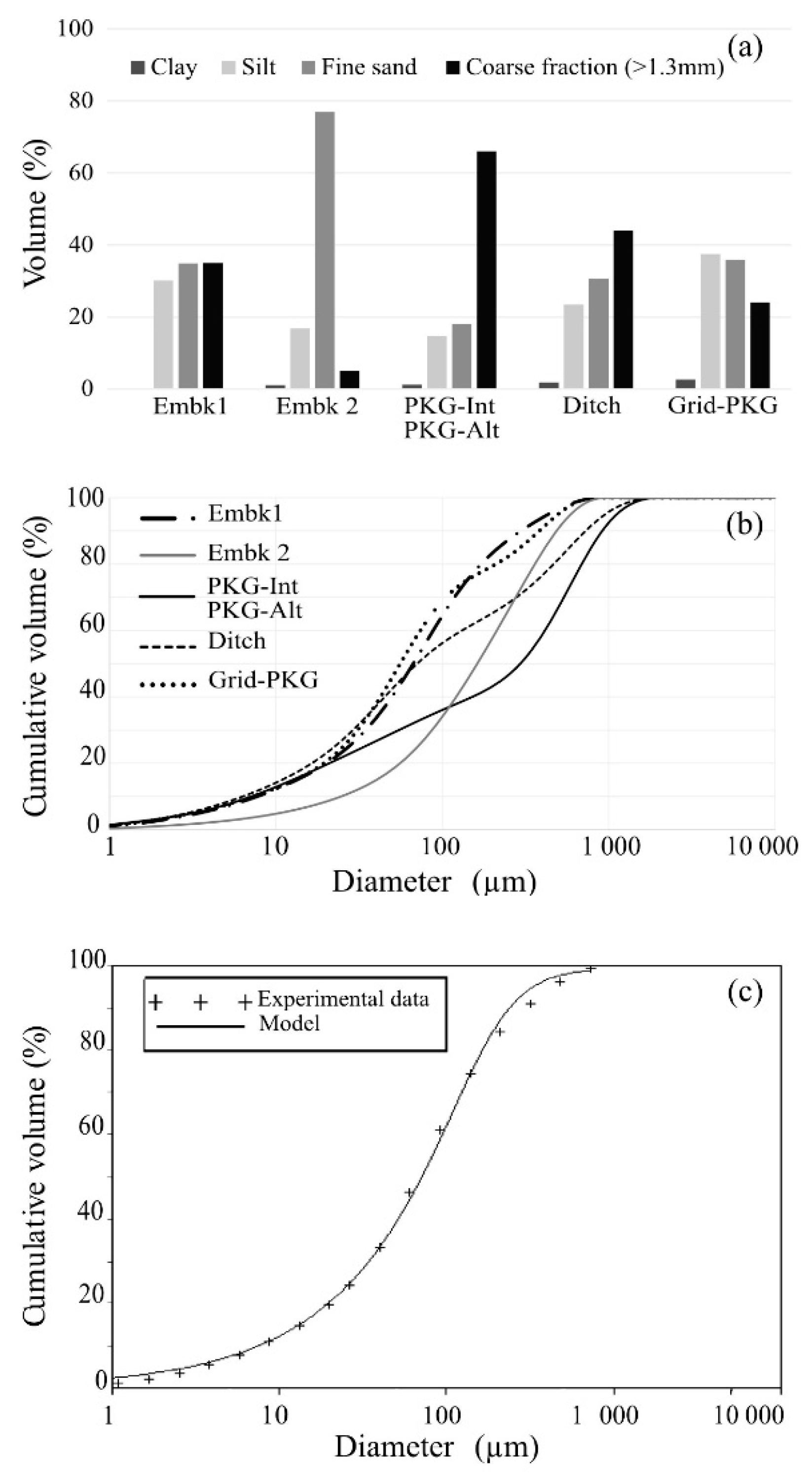
Shape Parameters from Particle-Size Analysis
Step-1: Fitting equation
F ( D ) = [ 1 + ( D g D ) N ] M (8) M = 1 2 N (9)F(D) is the cumulative frequency
D diameter
M and N shape parameters
Dg scale parameter
M, N and Dg are defined by optimizing the fit to the PSD (fraction < 1.3 mm) by the least square technique
Step-2: Solving for fractal dimension s
( 1 ε ) s + ε 2 s = 1 (10) κ = 2 s 1 2 s ( 1 s ) (11)s fractal dimension of media
ε soil porosity
Step-3: Shape parameters
m = 1 p m ( 1 + p m 2 1 ) (12) p m = m n 1 + m (13)pm shape index
m, n pore distribution index
p m = M N 1 + M ( 1 + κ ) 1 (14) n = 2 1 m (15)
η = 2 n × m + 2 + p (16) η hydraulic conductivity shape parameter
p tortuosity parameter *
(10) and (11) Fuentes et al. 1998 [30]; (12) and (13) Zatarain et al. 2003 [31]; (16) Haverkamp et al. 1999 [23]; * p = 1 (Burdine 1953) [21].
Table 2. Estimation of hydrodynamic parameters Ks and S by the Beerkan estimation of soil transfer parameters (BEST) methods using the model of Haverkamp et al. (1994) [32].
Axisymetrical infiltration model of Haverkamp et al. (1994)
I ( t ) = S t + ( A S 2 + B K s ) t (17) q ( t ) = S 2 t + ( A S 2 + B K s ) (18)
Constants A, B and C*
A = γ r d ( θ s θ 0 ) (19) B = ( 2 β ) 3 [ 1 ( θ 0 θ s ) η ] + ( θ 0 θ s ) η (20) C = 1 2 [ 1 ( θ 0 θ s ) η ] ( 1 β ) ln ( 1 β ) (21)
β ≈ 0.6 and γ ≈ 0.75 **
BEST methods
iexp steady state regression line slope
bexp steady state regression line intercept
BEST slopeBEST interceptBEST steady
K s = i e x p A S 2 (22) K s = C S ² b e x p (24) K S = C   i e x p   A b e x p + C (26)
I ( t ) = S t + [ A ( 1 B ) S 2 + S i e x p ] t (23) I ( t ) = S t + [ A S 2 + B C s ² b e x p ] t (25) S = i e x p   A + C b e x p   (27)
The Haverkamp equation fitting on experimental data allows to calculate the sorptivity S and subsequently the saturated hydraulic conductivity Ks.
* A, B and C defined under the Burdine et al. (1953) [21] condition [2] by the equations of Haverkamp et al. (1994) [32]; for the specific case of Brooks & Corey (1964) [22] equation [3]; ** β and γ values are valid for θ0 < 0.25 θs [33].
Table 3. Hydraulic shape parameters (n, m, and η) and shape parameter function cp.
nmηcp
Embk 12.360.158.612.06
Embk 22.330.148.972.09
PKG-Int2.260.1210.642.20
PKG-Alt2.260.1210.642.20
Ditch2.280.1210.082.17
Grid-PKG2.400.177.942.00
Table 4. Comparison of the observed infiltration rates to the obtained values of parameters Ks, S, and λm.
λm (mm)Ks (mm s−1)S (mm s−1/2)IR (mm s−1)Accuracy
BESTBESTBEST
slopeinterceptsteadyslopeinterceptsteadyslopeinterceptsteady
Embk 10.1020.1180.1390.0210.0250.0251.2901.3151.2110.108+
Embk 20.129 *0.155 *0.118 *0.0020.0030.0020.2820.2740.2480.012 *-
PKG-Int0.0590.0760.0870.0040.0060.0060.6720.6560.6160.025+
PKG-Alt0.1080.1260.1360.0370.0420.0431.4251.4081.3460.132+
Ditch0.0780.0710.0690.0360.0250.0331.4121.4961.2650.088+
Grid-PKG0.166 *0.213 *0.443 *0.011 *0.0070.0120.6190.7180.5850.031 *-
(+) Accurate (-) Inaccurate; * λm does not correspond to the observed IR.
Table 5. Normality test Kolmogorov–Smirnov on the estimates of Ks and S by the three BEST methods.
ParameterBESTNormalityLog-Normality
Dp-valueDp-value
Ksslope0.2410.0280.1110.736 *
intercept0.2360.0340.1140.711 *
steady0.2570.0160.0890.922 *
Sslope0.0840.946 *0.0980.861
intercept0.1100.749 *0.0880.926
steady0.0770.976 *0.1070.781
* p-value > 0.05 Distribution is normally/Log-normally distributed.

