Study of the Scale Effect on Permeability in the Interlayer Shear Weakness Zone Using Sequential Indicator Simulation and Sequential Gaussian Simulation

Abstract

The interlayer shear weakness zone (ISWZ) is a deformation zone in stratified rock masses, with different width and spacing, due to tectonic stresses. It represents the main flow path in rocks due to higher permeability compared with massive rocks. The permeability values of an ISWZ can vary significantly depending on the scale. This study focuses on the correlations between the permeability properties of ISWZs and their geometry properties. A range of realistic 3-D numerical models of ISWZs is developed using geostatistical modeling, with fine-scale geometry and permeability information taken into consideration. These ISWZs represent a set of mud content and width distributions that are typical for ISWZs. Horizontal and vertical permeability values for all ISWZs are found to change in small-scale samples, whereas these fluctuations decrease with increasing sample size. For different types of ISWZs, the results show that ISWZs with variable width will show a significantly larger scale effect on the permeability than that of ISWZs with constant width. Furthermore, ISWZs with a higher mud content display greater variation in horizontal permeability, while the opposite is true for vertical permeability. Based on the coefficient of permeability variation, a criterion is proposed to identify the calculated permeability of a sample is locally homogeneous. The size for this sample relies on the properties estimated (horizontal and vertical permeability) and geometry features. These findings could provide a basis for the selection of permeability values of an ISWZ in hydraulic engineering. Additionally, the procedures used in this article can be applied to any type of ISWZs.

1. Introduction

Most rocks possess discontinuities (such as fractures, faults and shear zones) which facilitate groundwater flow through them. However, some discontinuities (such as faults and dykes) may act as a barrier to fluid flow [1]. The permeability characteristics of rocks depend on both the intact rock formations and their discontinuities [2,3,4]. It is therefore extremely important to quantify the hydrogeological properties of discontinuities in rocks.

As regards volcanic rock masses, individual strata of basalt resulting from multiple distinct eruptions may be interlayered with tuffs. Where tectonics stresses the masses, brittle shear planes may develop especially close to the contact between basalt and tuff. The interlayer shear weakness zones (ISWZ) formed from the dislocation of the tuff is characterized by a weaker shear strength and a higher permeability compared with massive rocks [5,6,7]. As a result, an ISWZ may generate several issues in hydraulic engineering, such as: dam breaks, water inrush in underground chambers, slope instabilities, seepage deformation of ISWZs and leakage in the reservoirs and dam foundations. Thus, it is necessary to describe the geometric features of ISWZs and study their hydrogeological and mechanical properties. Xu et al. [5] adopted a dynamic method by regarding an ISWZ as a joint filled by interlayer soil with varying width and developed a shear strength model to describe the shear behaviors of interlayer soil. Cui et al. [6] analyzed the impacts of near-fault ground motion on discontinuities, and the C₂ was selected as an example, which is one of ISWZs developed in the Baihetan dam site, to describe the discrepancy between near-fault ground motion.

In order to study the hydrogeological characteristics of structural planes, such as ISWZs and faults, scholars have conducted various studies. It is possible that shear faults have multiple parallel shear zones, where fractured surrounding rocks and primary lenticels can be found above and below [8]. Caine et al. [9] and Cleary et al. [10] studied the permeability relationships between the shear zones and crushed zones, and found that the permeability values of the former are much greater than those of the latter. However, increased fracture development of the crushed zone of wall rocks correlates with increased permeability. Therefore, the role of the crushed zone cannot be neglected for the flow characteristics analysis of fault zones. Jourde et al. [11] described the shear zone in sandstone and studied the transmissivity ecoefficiency of fault zones, based on the permeability of both shear zones and crushed zones. Numerical simulation methods in hydraulic characteristics regarding fault zones are abundant [12,13,14,15,16,17]. These methods treated the fault as a collection of a number of fractures with varying sizes in hydraulic simulation. Bonnet et al. [18] conducted fault-zone hydraulic simulation based on the development of the water flowing fractures, and used discrete element methods to analyze the scale effect on the fault-zone seepage performances. This study showed that the permeability values of fault zones tend to be stable when the scale reaches 50 m. Based on in-situ permeability data from borehole experiments and careful statistical studies, Figueiredo et al. [19], Jiang et al. [20] and Sanford et al. [21] found that the permeability values of fractured surrounding rocks decrease with depth.

Maryška et al. [22] established a stochastic discrete fracture network model, and then adopted a numerical method to simulate fracture flow. Malkovsky’s et al. [23] and Hanor’s et al. [24] found that the average permeability of fault zones is two orders of magnitude larger than their minimum permeability. Therefore, the average permeability values calculated at the scales greater than 50 m are more representative when continuity has been affected. Shipton et al. [25] and Fourno et al. [26] determined the hydraulic conductivity structure of fault zones based on the stress distribution of the area. Various statistical algorithms based on geology are commonly used in geometry and permeability modeling of a heterogeneous porous medium. The porous medium itself is usually regarded as a discrete variable, and it is usually retrieved using the sequential indicator simulations (SIS), transition probability geo-statistics (TPROGS) and indicator kriging (IK) [27,28,29]. Petrophysical parameters are always simulated by the Monte Carlo (MC) and sequential Gauss simulations (SGS) as they are usually viewed as continuous variables [30,31,32]. The SGS is regarded as the preferred method for simulating continuous variables. The best characteristic of this algorithm discussed is that the variables simulated by SGS conform to a normal distribution, and it only needs two parameters to determine the distribution feature of variables. The SIS is a stochastic simulation, first proposed by Journel et al. [33], that can be used in both discrete variables and continuous random variables. This simulation method is advantageous because it can simulate more complicated anisotropic geological phenomenon relative to traditional algorithms. For variables with discontinuous distributions, such as the fillings of an ISWZ, it can establish anisotropic simulation results since they are represented by different variograms.

From a hydrologic perspective, ISWZs can be regarded as being filled by the low-permeability fillings (mud and debris) and the high-permeability fillings (gravel and fractured surrounding rock). The estimation of the permeability for such ISWZs as a function of scale is studied by computing the effective permeability of ISWZs on different scales. The study varies in approach relative to several previous studies [34,35]. These studies established correlations between the structural-plane geometry properties and the permeability properties in terms of a few relevant parameters. In the present article, detailed geometry information of ISWZs is described by their geometry models which are developed by the SIS. The basic input parameters of a geometry model are obtained by analyzing the centimeter-scale resolution field image which distinguishes the spatial distribution features of each filling. Moreover, previous studies have commonly treated the permeability values of the same medium as a constant value; however in reality, their permeability values can also vary up to 1–2 orders of magnitude. The SGS has been adopted here to generate 3-D permeability models, allowing each filling’s permeability values to have a non-fixed value but limited to a log-normal distribution. The permeability values of the fillings in this article are measured through field and laboratory tests and are then subsequently are inputted into the permeability model of an ISWZ.

2. Materials and Methods

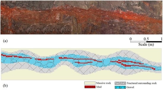
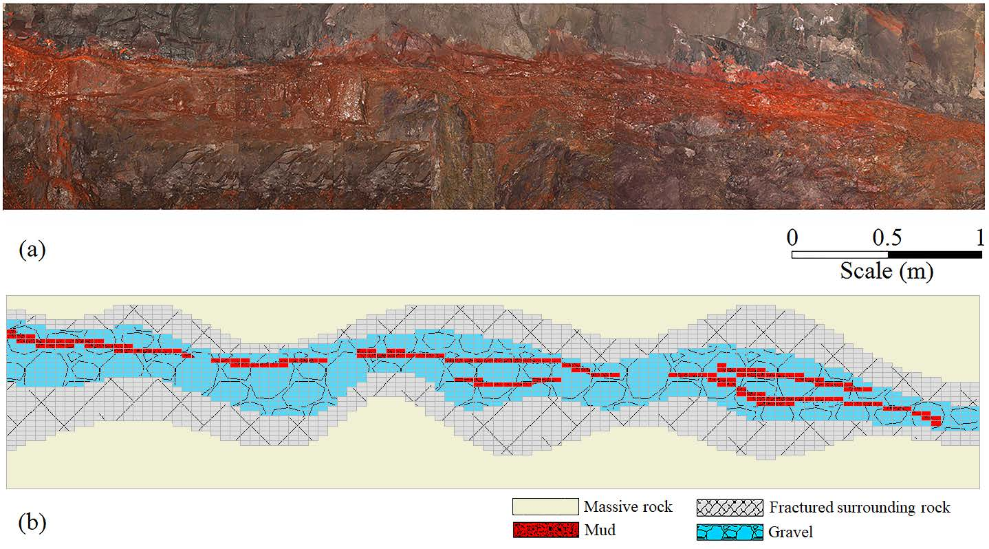
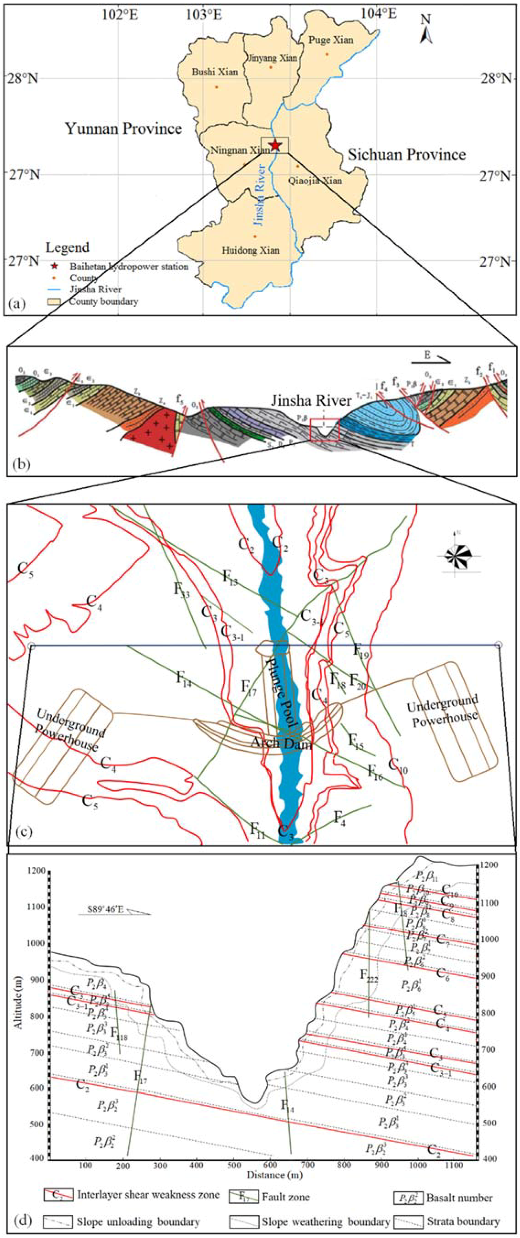
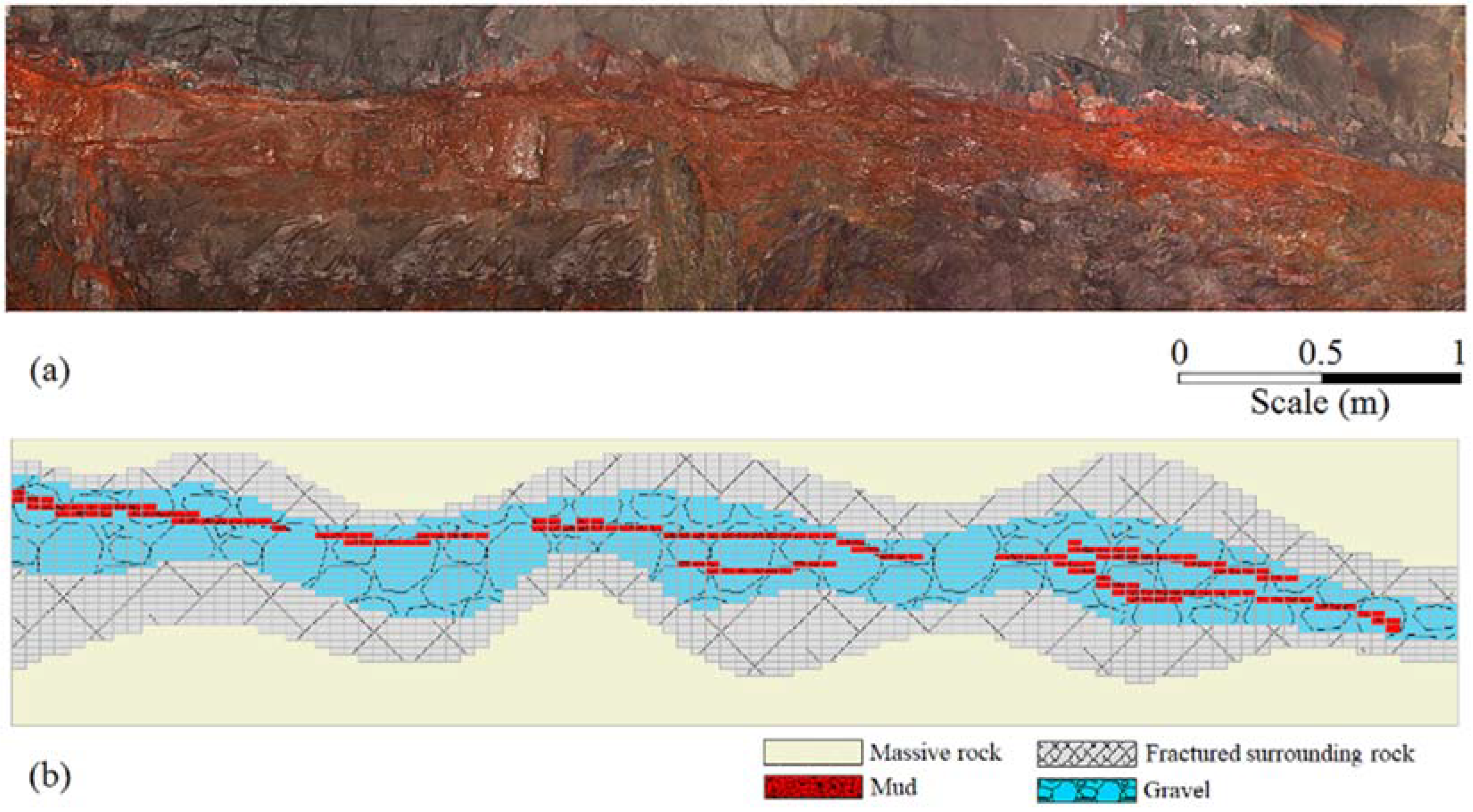
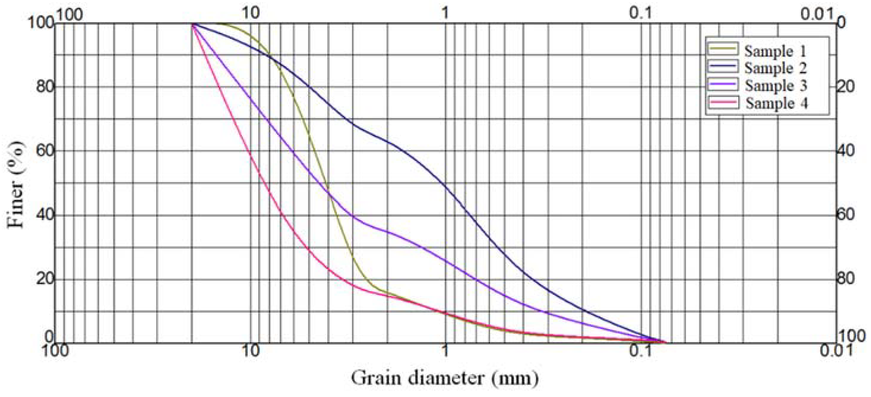
2.1. General Description of the Interlayer Shear Weakness Zones

The interlayer shear weakness zones (ISWZ) shown in Figure 1 are developed on both sides of the mountains of the Baihetan dam site. This indicates that ISWZs tend to present a continuous and extensive distribution in basalt. The Baihetan dam site is located at the Jinsha River Basin in southwest China, and offers the second largest average annual power production in the world. The site includes an arch dam 289 m high, several drainage galleries, two main underground powerhouses (440 m long, 30 m wide and 33 m high) and 229 tunnels (65 km long in total). The Jinsha River is 2316 km long and flows through the Sichuan basin. The flow speed of the Jinsha River is very fast as it adheres to the geological conditions of high mountains around a deep valley. The water level in the reach of the Jinsha River has a difference of 3300 m, and its hydropower resources can create more than 110 million kilowatts of power.

The rock masses under the construction of the Baihetan dam are primarily Emeishan (P₂β) basalts of the Upper Permian. Basalt is an igneous rock, formed from the cooling of lava erupted from the upper mantle. The rock units have been folded into a monocline, which gently dips (S120–145E/15–20, dip direction/dip) towards the right bank of the upstream section [36,37]. At the Baihetan dam site, eleven lava flows (P₂β₁–P₂β₁₁) have been noted, each separated by a discontinuity produced by time between distinct eruptions. In general, an incompetent tuff layer composed of basaltic debris, basaltic gravel and other sediments is found between each lava flow, with a width no more than 1 m. Subsequent tectonic stress has folded the rock strata into a series of folds. During the formation of these folds, structurally complicated ISWZs were formed in the incompetent tuff layers as a result of shear dislocation. The ISWZs on the left bank of the Baihetan dam site contain C₂, C₃ and C_3-1. However, the right bank contains C₂ to C₁₀. Geological surveys reveal that different ISWZs present varying degrees of dislocation, with argillisation appearing in some regimes affected by groundwater. The mud-dominated sections of individual ISWZs are impermeable, consequently fluid flow is concentrated along gravel-dominated layers. This phenomenon indicates that permeability within ISWZs is controlled by strong heterogeneity and anisotropy.

The ISWZ is a special structural plane which is composed of low-permeability components (mud and debris) and high-permeability components (gravel and fractured surrounding rock). Figure 2 shows that the massive rock is intercalated with fractured surrounding rock, mud, debris and gravel, often in lenticular, laminated and wavy shapes.

Field scanline surveys of ISWZs in the Baihetan dam site show that ISWZs are found to have different widths at different locations due to variable development intensity. The distribution and particle size of the fillings are not uniform; however, they conform to some geological rules. The fillings in an ISWZ display a good stratification (see Figure 2). The grain-size distribution of C₃ (see Figure 3) denotes that the grain size of interlayer soils has a broad distribution, ranging from 0.075 mm to 20.0 mm.

With regards to the grain size of the fillings, they can be divided into four categories based on the Chinese National Standards GB 50287-2006: mud, gravel, debris intercalated with mud, mud intercalated with debris. In practice, it is impossible to distinguish between mud, debris intercalated with mud and mud intercalated with debris. In addition, we found there is little difference between their permeability values by analyzing test statistical data. Therefore, this study merges these three categories into a single type, namely mud. Additionally, tectonic activities and local stress concentrations cause slight to strong unloading of massive rocks on both sides of ISWZs. This unloading always contributes to a more fractured development in massive rocks; as a result, there is a larger permeability in massive rocks relative to the fresh bedrock. Thus, the flow impacts of fractured surrounding rocks should not be ignored following analysis of permeability properties of ISWZs. In summary, the fillings in the ISWZ are classified into three categories: intercalated mud, gravel and fractured surrounding rock. For places with a moderate degree of dislocation, a large amount of gravel begins developing in ISWZs, which results in enhanced permeability of an ISWZ. For strongly dislocated and weathered locations, the fillings in ISWZs have the highest degree of fragmentation. As a result, the permeability of this ISWZ is the strongest and continuous dripping may occur in some locations. Therefore, with the increase of gravel content in an ISWZ, its permeability enhances gradually. It should be noted that enhanced permeability may also encourage argillization in debris under the physical and chemical reactions of groundwater.

2.2. Basic Principles and Methods of Modeling

In this study, we first employ the SIS to generate the 3-D geometry model of the ISWZ. The SGS then is adopted to create the 3-D permeability model. Whichever inversion method is applied, the key is to estimate the LCPD (local conditional probability distribution) of each grid point. SIS was first proposed by Journey [33] and was regarded as a useful approach to retrieve cm-scale stochastic variables. As a typical of sequential indicator simulations, SIS is applicable to retrieving both continuous and discrete variables. Moreover, SIS does not suffer any limitations from the normal distribution hypothesis and determines the distribution of random variables by predicting, through a series of threshold values, the probability in which one variable might be lower than a certain threshold value. The key to the accomplishment of SIS is indicator transformation, indicator kriging and sequential simulation. Before simulation, indicator transformation should be performed, which means to encode original data as 0 or 1 by following different threshold values. Suppose Z(x) is the parameter value at X; then, the indicator transformation for those with a threshold value of Z₀ might be expressed as follows:

$$I\left(Z_0,Z\right)=\{\begin{array}{l}1,Z\le Z_0\\ 0,Z>Z_0\end{array}$$

(1)

Suppose the exterior condition remains unchanged in observing variable Z; then a much larger value of Z_i (i = 1, 2, 3, …, n) can be obtained after observing the variable Z n times. Under such circumstances, the ratio of the number of Z_i < Z₀ to n can show the probability of Z < Z₀. During practical geological study, only one observed value is, in most cases, selected for one variable at a certain point. Moreover, a random process should be assumed to be second-order stationary. For these reasons, when the sample capacity n is quite large, the probability of Z < Z₀ can be calculated by the ratio of the number of Z_i ≤ Z₀ to n, namely:

$$F\left\{Z_0,Z|(n)\right\}=P\left\{Z\le Z_0|(n)\right\}=\frac{1}{n}{\displaystyle \sum _{i=1}^{n}I\left(Z_0,Z_i\right)}$$

(2)

Furthermore, indicator transformation can be also applied to variables. For each type of filling within the simulation target zone, when it appears at some location, the indicator variable should be either 1 or 0 (when other types of the filling exist, the indicator for the filling will be 0). Therefore, the information of different types and varying accuracy can be transformed into 1 and 0 to synthesize the data. SIS usually adopts indicator kriging to estimate the LCPD. As opposed to other kriging methods, indicator kriging is mainly for indicator prediction. Weight will be given according to the location and loading of the sample. At this point, Equation (2) can be transformed into:

$$F\left\{x,x|(n)\right\}={\left[I\left(z,x\right)\right]}^{\ast }={\displaystyle \sum _{i=1}^n{a}_i\left(z,x\right)\cdot I\left(z,x_i\right)}$$

(3)

where [I (z, x)]* is estimated value while a_i (z, x) is weight.

a_i (z, x) can be solved by the following equations:

$${\displaystyle \sum _{i=1}^n{a}_i\left(z,x\right)\cdot C_1\left(z,x_i-x_j\right)+\mu \left(z,x\right)=C_1\left(z,x-x_i\right)\left(j=1,2,\cdots ,n\right)}$$

(4)

$${\displaystyle \sum _{i=1}^n{a}_i\left(z,x\right)}=1$$

(5)

For some locations, each threshold value must have a corresponding equation. Within the change range of variable Z, the range can be discretized by K threshold values. Hence, only when K equations are solved can the solution to F {Z_k, x|(n)} (the cumulative distribution function) be obtained. The cumulative distribution function value between [Z_k, Z_k+1] can be achieved by means of linear interpolation. In this way, the LCPD at all locations can be determined. When SIS is applied to conducting a conditional simulation for K discrete variables (S_k (k = 1, 2, 3, …, K)), the following steps can be followed:

(1)

Transform the discrete variable S_k into an indicator variable. Set i_k (u) as the indicator value of S_k. When u ∈ S_k, i_k (u) is 1, otherwise it is 0. For all samples, K discrete variables must be mutually exclusive. In other words, the following relations can be established:

$$\begin{gathered} i_k(n)i_k^{\prime }(n)=0,\forall k\ne k^{\prime } \\ {\displaystyle \sum _{k=1}^k{i}_k(u)=1} \end{gathered}$$

(6)

(2)

Calculate the indicator variation function of each indicator variable i_k (u). If there is a cluster effect for the original data, the cluster effect should be eliminated first.

(3)

The following steps should be used to conduct sequential simulation:

(i)

Determine the random access path for each grid point. Confirm the quantity (maximum and minimum) of the adjacent conditional data (including the original y and the y value of the grid point) at appointed grid point.

(ii)

Apply indicator kriging to the indicator variable i_k (u) to estimate the probability that the type variable at the grid point belongs to S_k. For example, when simple indicator kriging is used, the probability of S_k at grid point u is:

$$P^{\ast }\left\{I_k(u)=1|(n)\right\}=P_k+{\displaystyle \sum _{\alpha =1}^n{\lambda }_{\alpha }\left[I_k(u_{\alpha })-P_k\right]}$$

(7)

where P_k = E{I_k (u)} ∈ [0, 1] is the marginal probability which can be inferred. The weight coefficient λ_α can be obtained through the simple kriging equations.

(iii)

Determine the sequence (e.g., 1, 2, 3, …, K) of k discrete variables S_k. This sequence defines the distribution order of k discrete variables S_k within the probability range of [0, 1].

(iv)

Randomly formulate a value within [0, 1] and determine the type of the discrete variable corresponding to the value. This type refers to the variable type of the grid point.

(v)

Use a simulated value to update the k indicator data set and deal with the next grid point by following a random path until all the points have been simulated. Under such circumstances, one realization is obtained.

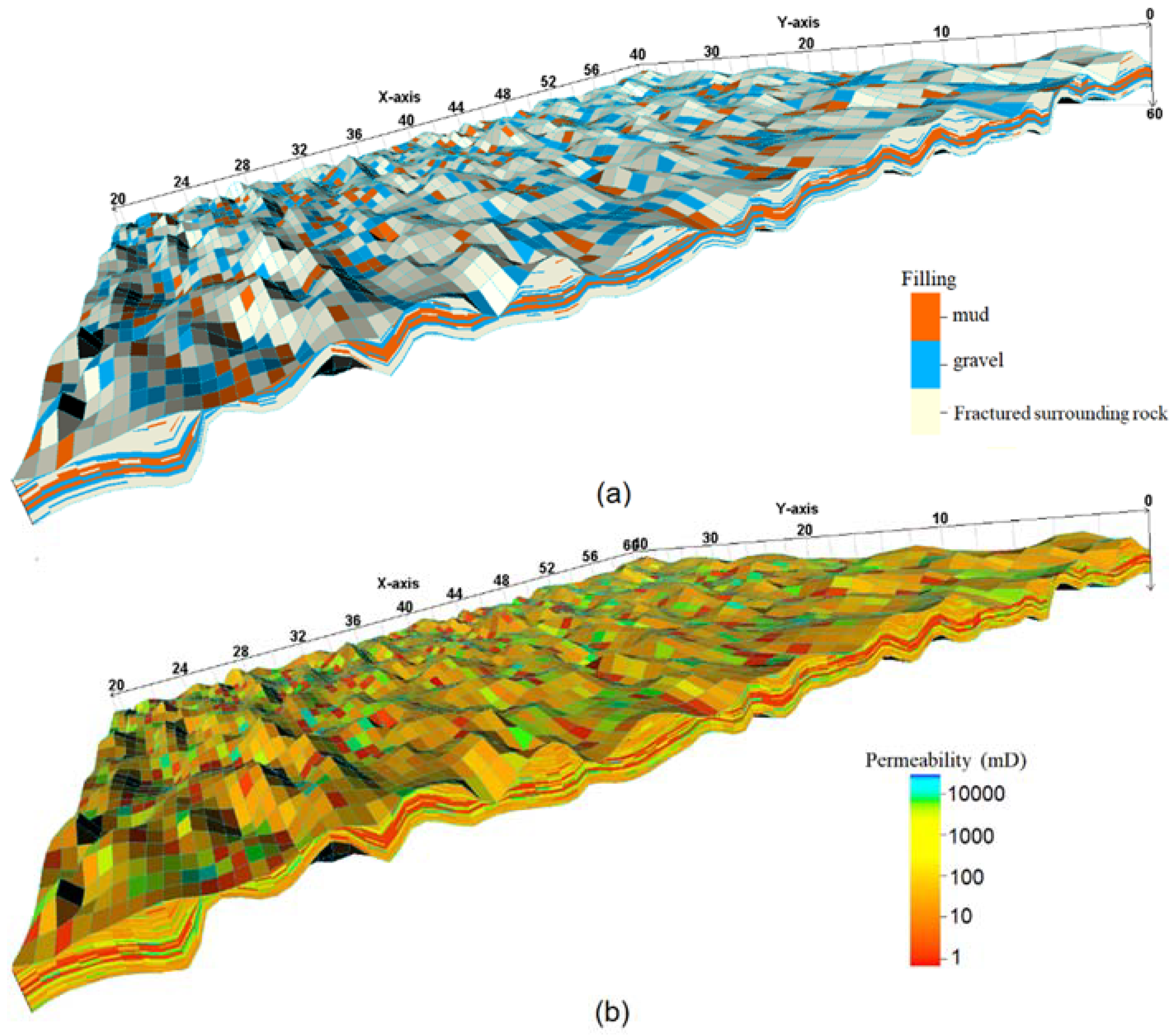
2.3. Generation of the 3-D Numerical Models

In this study, the numerical models of ISWZs are generated based on the various input parameter groups listed in

Table 1. Main input parameter groups adopted to generate a numerical model.

Geometrical Input Parameters	Permeability Input Parameters
ISWZ width (range, mean and standard deviation)	Mud permeability (range, mean and standard deviation)
Fillings percentage	Gravel permeability (range, mean and standard deviation)
Variogram parameters (major and minor range, search radius, etc.)	Fractured surrounding rock permeability (range, mean and standard deviation)
SIS parameters (distribution type and distribution parameters)	SGS parameters (distribution type and log-normal distribution parameters)

.

The 3-D geometry model is developed by the approaches of kriging interpolation and SIS, and the corresponding permeability model is retrieved using SGS. The detailed features of an ISWZ are included in these numerical models. Five realizations are considered for each ISWZ, and each realization includes the same geometry and permeability information.

2.3.1. The Geometry Model

To describe these fine-scale geometry characteristics of an ISWZ, a geometric model should be generated first. In practice, the width of different ISWZs may follow multiple laws of normal distribution (see

Table 2. The width distribution laws for partial ISWZs which are developed in the Baihetan dam site.

Type	Normal Distribution Parameters of the Width (cm)
	Minimum	Maximum	Mean	Standard Deviation
C2	12.9	58.3	31.49	7.5
C3	14.3	108.8	44.12	15.6
C4	14.1	102.1	61.86	14.6
C5	27.3	65.4	46.8	6.3

).

It is therefore impossible to study all the distribution conditions of the width. Field scanline surveys (including record the distribution features of the fillings and the width distribution of ISWZs) show that the width of all ISWZs in the Baihetan dam site varies in most locations from 10 cm to 100 cm. Therefore, there are two extreme cases of width distribution to be considered in this study: constant width (100 cm) and varying width (10–100 cm). For the models with varying width, all types of ISWZs studied in this article accord with the same standard normal distribution (i.e., standard deviation is 15). Additionally, we found that the percentage of fractured surrounding rocks in all ISWZs have a small change from 30% to 40%. In order to facilitate the study, the content of fractured surrounding rocks of each ISWZ is assumed to remain unchanged 30%, and an ISWZ is gradually filled by mud from 10% to 60%. To study the correlations between the permeability properties of ISWZs and their geometry properties, eighteen types of ISWZs are generated in this study. These ISWZs represent different width distributions and filling content.

Table 3. Main geometry parameters for all the studied ISWZs.

ISWZ Type		Mud Content (%)	Distribution Parameters of the Width (cm)
			Range	Mean	Standard Deviation
Constant width	Type1	10	100	100	0
	Type2	20	100	100	0
	Type3	25	100	100	0
	Type4	30	100	100	0
	Type5	35	100	100	0
	Type6	40	100	100	0
	Type7	45	100	100	0
	Type8	50	100	100	0
	Type9	60	100	100	0
Varying width	Type10	10	10–100	55	15
	Type11	20	10–100	55	15
	Type12	25	10–100	55	15
	Type13	30	10–100	55	15
	Type14	35	10–100	55	15
	Type15	40	10–100	55	15
	Type16	45	10–100	55	15
	Type17	50	10–100	55	15
	Type18	60	10–100	55	15

lists the geometry parameters of all the studied ISWZs in this article. Considering the uncertainty of modeling, each geometric model for an ISWZ achieves five realizations, so eighteen geometric models, ninety realizations are generated in total.

Geometry parameters inputted in the geometric model of an ISWZ should include these fine-scale geometry characteristics as they have a great influence on the hydrological properties. If there is a good match between the geometry input parameters and the measured geometry data, a set of realistic realizations would be developed. Figure 4 shows one realization of an ISWZ which has a mud content of 30% (Type 13), and its geometric model is shown in Figure 4a. Still, there are a few limitations to this approach; for example, it is impossible to include all natural variability of the fillings into the geometric model.

2.3.2. The Permeability Model

The permeability model is a detailed description of the permeability information of the fillings. As shown in Figure 5, the difference in the permeability can be as large as four orders of magnitude for different fillings (between mud and gravel).

Moreover, even for the same filling, there will be a difference up to one-two orders of magnitude, and the permeability values of each filling are basically in conformity with logarithmic normal distribution. This point, despite its limited sample data, confirms the result of Freeze [38] who discovered through a great deal of permeability statistics that permeability usually follows the rule of logarithmic normal distribution.

Table 4. Permeability results of the fillings in ISWZs.

Fillings	Log-Normal Distribution Parameters of Permeability (mD)
	Minimum	Maximum	Mean	Standard Deviation
Mud	0.7	5.6	2.1	0.8
Gravel	276.7	28,913.2	3818.5	3464
Fractured surrounding rock	16.5	605.3	119.8	78.9

gives the related permeability distribution parameters of the fillings in ISWZs, which are obtained by field and laboratory permeability test in the Baihetan dam site.

In employing SGS to develop the permeability model of an ISWZ, only when the permeability input information of the fillings is similar to their measured permeability data can the generated permeability model accord with the real situation (see Figure 5). Figure 4b shows a realization of the permeability model which has a mud content of 30% (Type 13). Additionally, each grid unit in Figure 4 has a fixed horizontal dimension of 0.1 × 0.1 m. However, as the ISWZ width varies, the longitudinal size of each grid is related to the width of different locations. For each grid, it should also be noted that it is assigned a certain permeability value depending on the type of the fillings it belongs to.

There are still some limitations to this method. First, the more test data obtained, the greater the likelihood of capturing the detailed permeability information of the fillings. Thus, there should be a sufficient amount of permeability test data. Secondly, permeability results of the fillings obtained from laboratory test tend to overestimate the permeability value as it is difficult to collect an undisturbed sample. Finally, identifying the permeability distribution parameters (e.g., the mean and variance) of each filling would be impossible. However, the approaches used in this article are considered to be acceptable for generating realistic geometry and permeability models as they have captured the most important factors which have great impacts on the permeability properties of an ISWZ.

3. Results

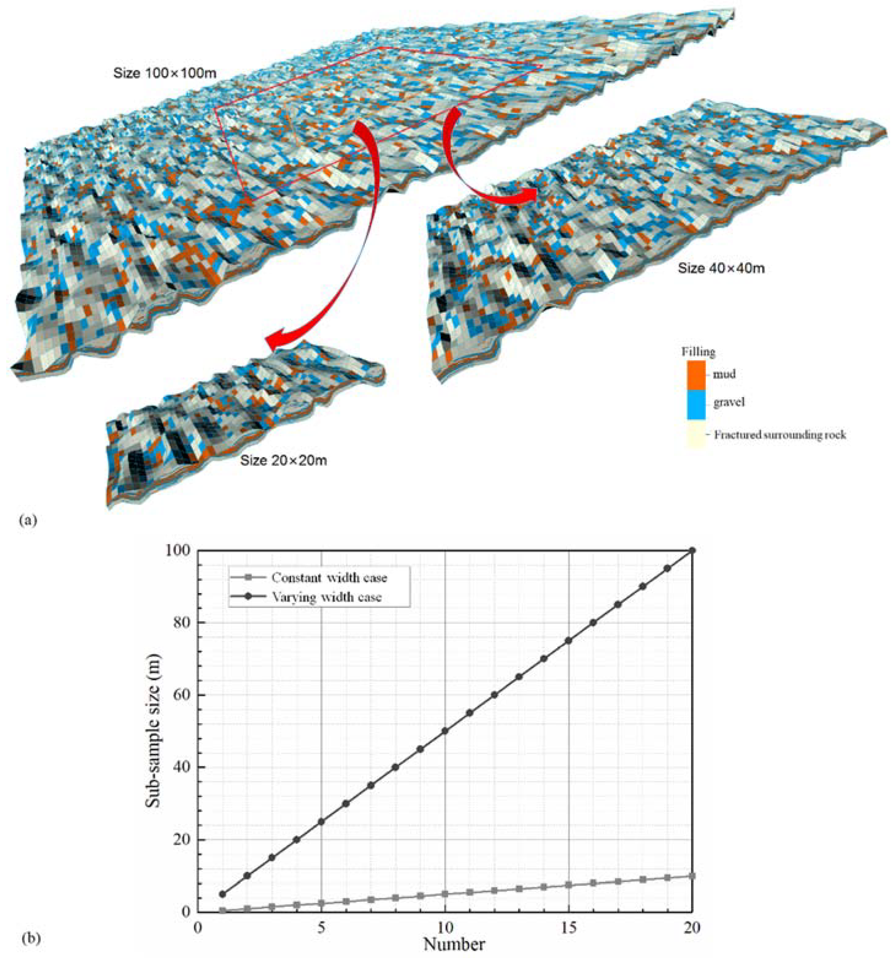
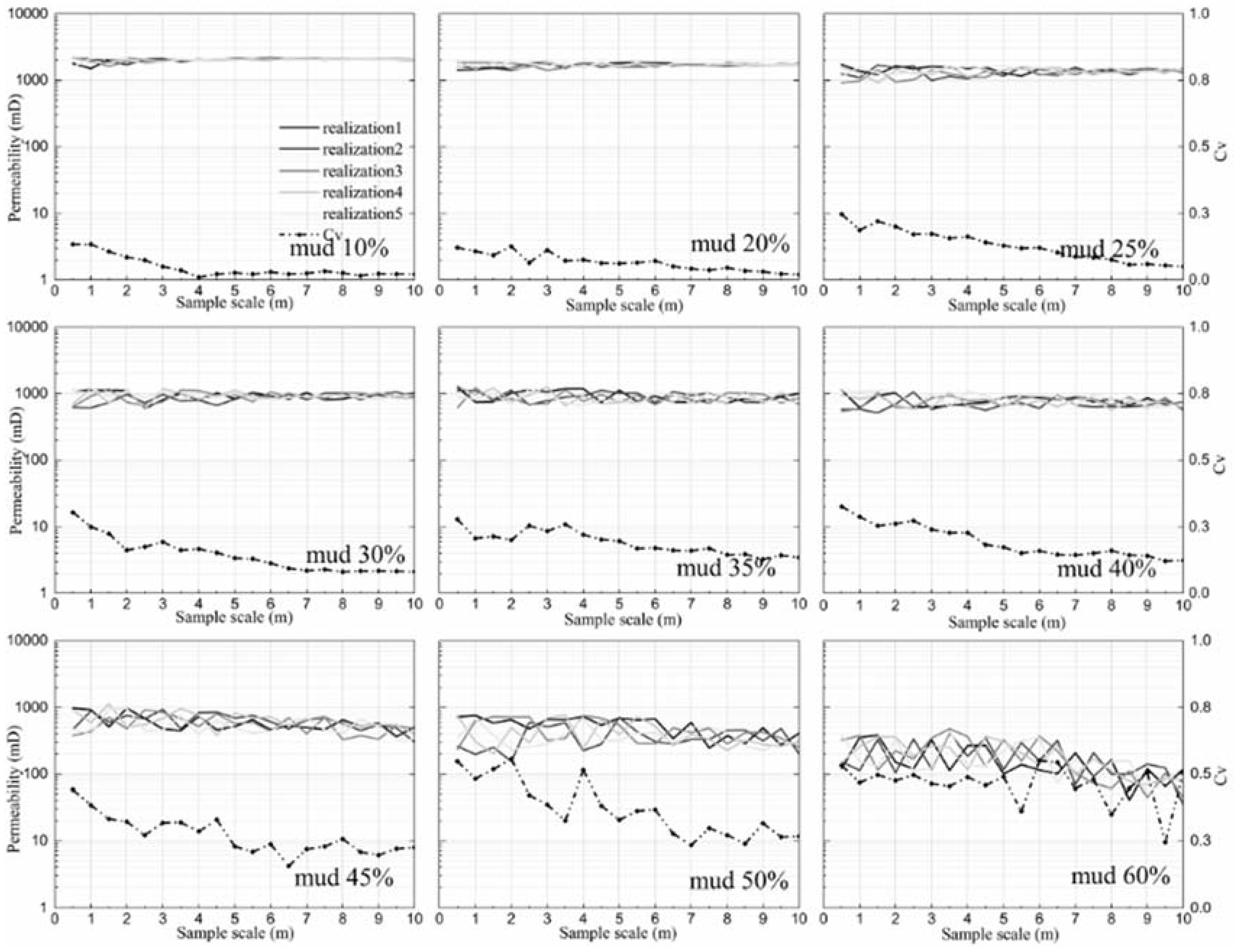
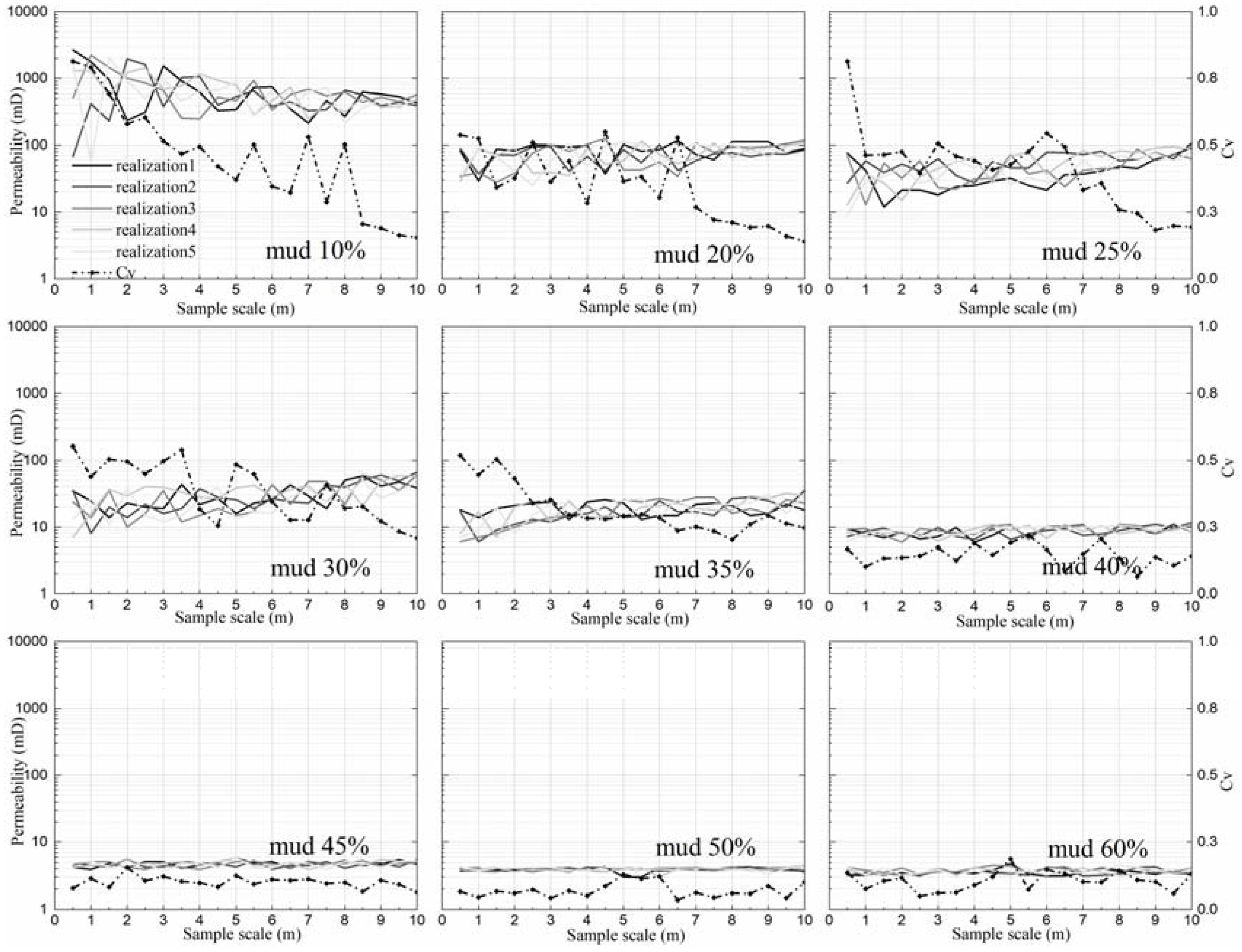
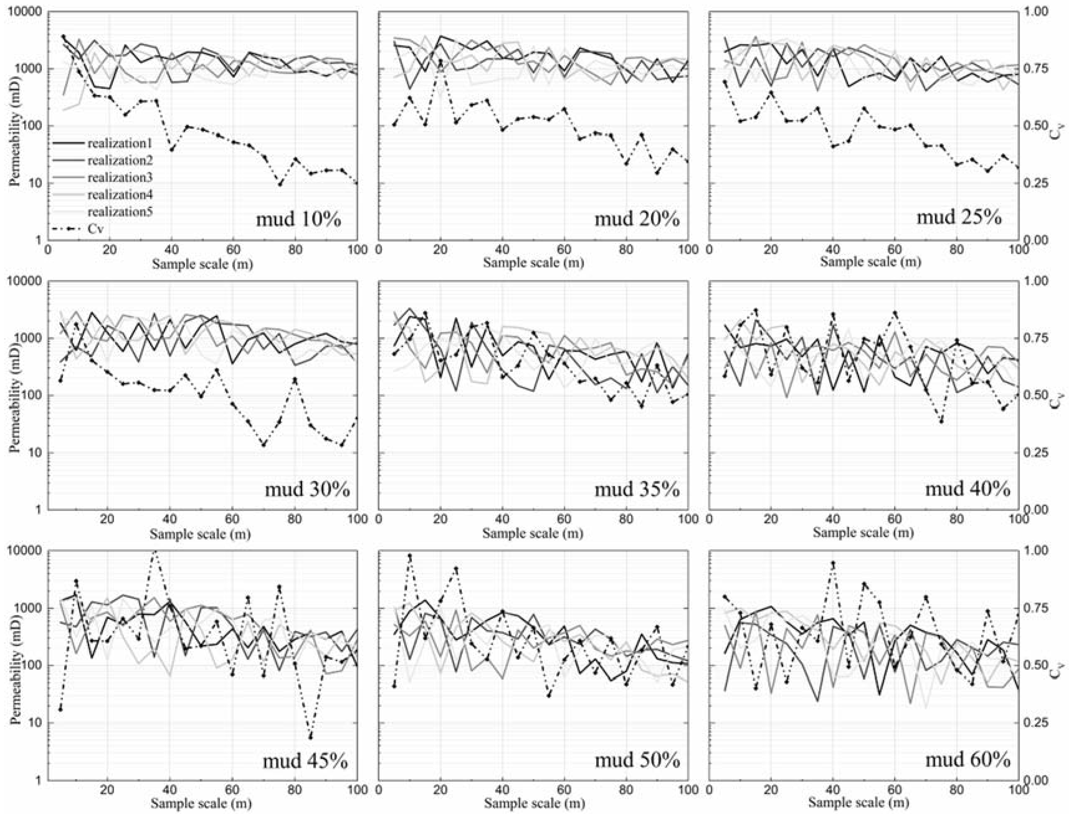
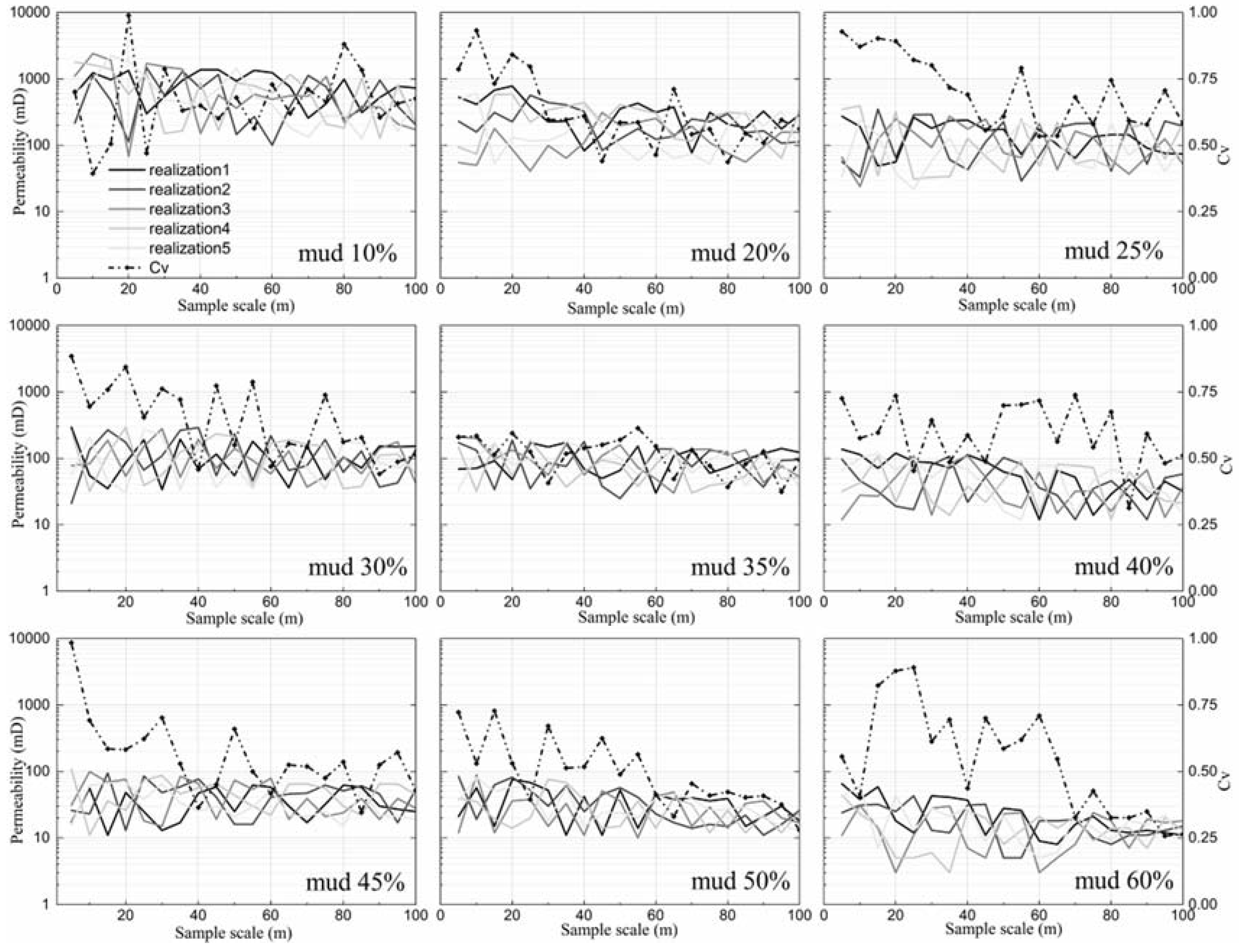
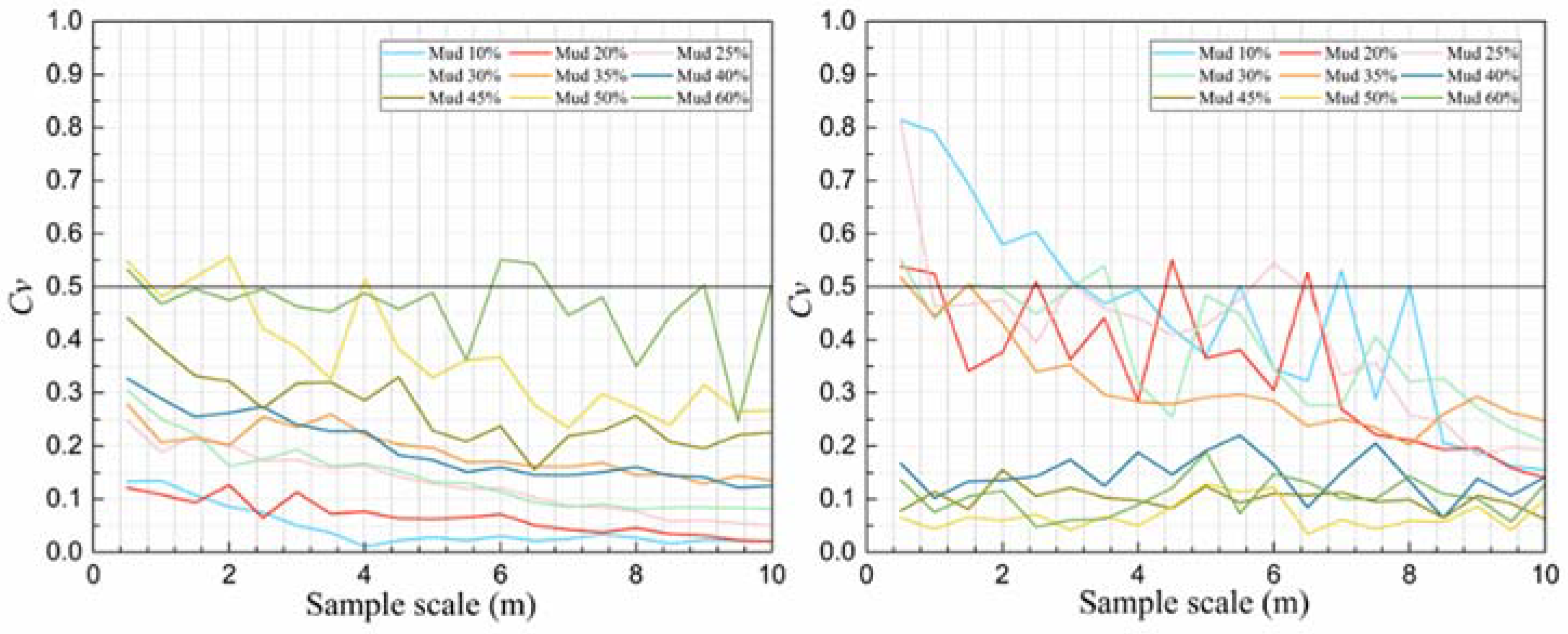
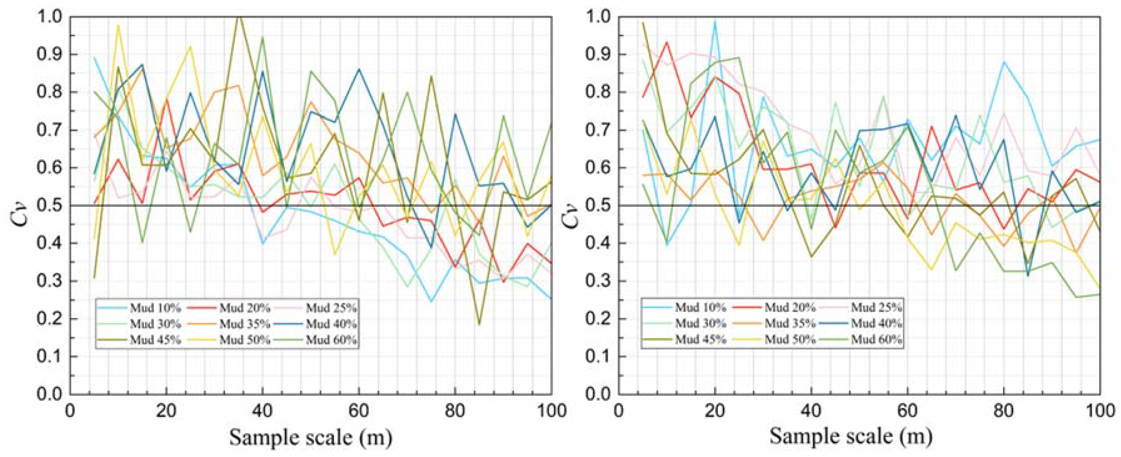
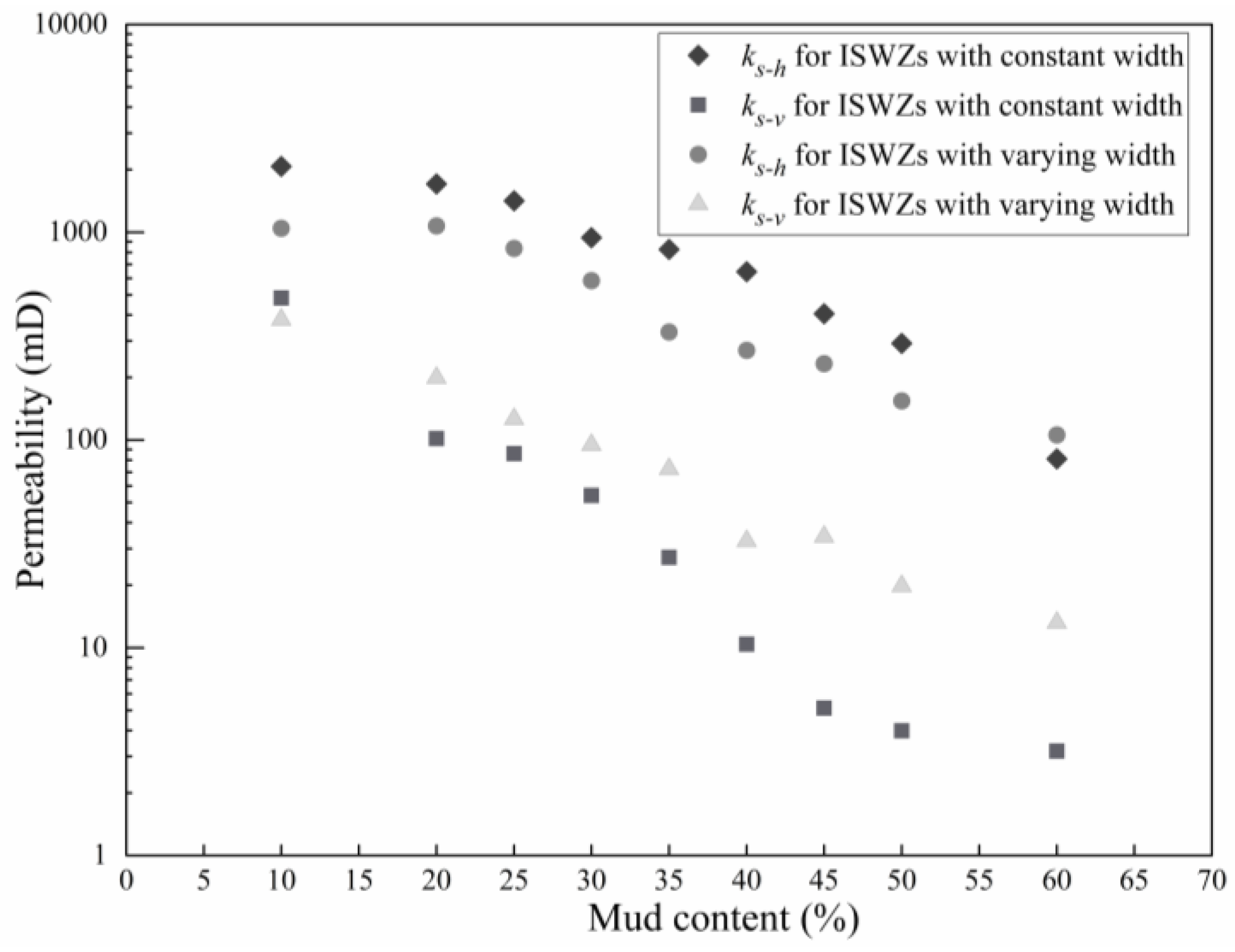
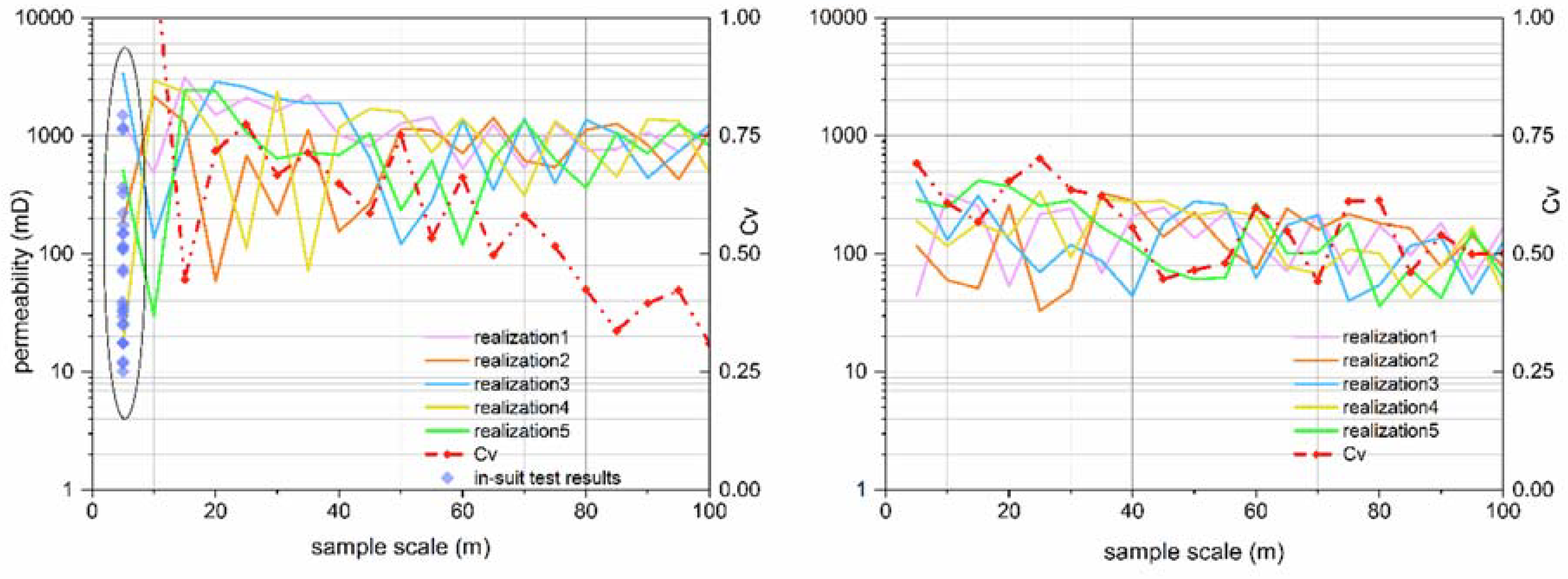
3.1. Variation of Permeability as a Function of Sample Support

As shown in Figure 6, in order to study how permeability varies with the sample scale, the sample was regularly extracted from each realization, in which sample scale was increased in 20 steps from the smallest scale (0.5 m for the constant width case, 5 m for the varying width case) at the center of the realization to the full model scale (10 m for the constant width case, 100 m for the varying width case).

The permeability of samples may range by several orders of magnitude with the enlargement of sample size, and the standard deviation is not high enough to estimate the permeability variation as it usually increases with the average permeability increase. If a particular sample has captured local homogeneity, that is, its permeability tends to be stable, this stable permeability is called the “representative effective permeability of an ISWZ (k_s)” and the corresponding size of this sample is called the “volume of the locally homogeneous region (V_s)”. However, it is difficult to identify whether a sample has captured local homogeneity. Corbett and Jensen [39] proposed that Cv is a persuasive parameter, which can be used to quantize the variability of permeability. The Cv, a normalized standard deviation that can be considered a normalized treatment of the deviation for a probability distribution, giving the proper estimator of the variation in permeability. The Cv can be expressed as:

$$Cv=\frac{\sigma (k)}{\overline{k}}$$

(8)

where σ(k) and $\overline{k}$ are the standard deviation and arithmetic mean of permeability between five samples.

According to the generalization of a large amount of permeability statistical data from many outcrops in the heterogeneous porous media, Corbett and Jensen [39] provided a means of classifying Cv values to quantify the degree of heterogeneity as follows: Cv < 0.5 indicates statistically homogeneous; 0.5 < Cv < 1 is regarded as heterogeneous. Instead of identifying k_s and V_s by only one realization, we propose a criterion based on Cv between the five realizations to estimate them. Note that a value of Cv < 0.5 may accidentally appear in a small-scale model, but only the scale in which the Cv remains below 0.5 is deemed valid. Jensen et al. [40] has a detailed discussion of Cv.

For highly heterogeneous porous media like ISWZs, the effective permeability must be calculated using a numerical method instead of an analytical method. Based on the permeability model of an ISWZ at different scales (see Figure 4b), a method by imposing an unchanged pressure gradient between the opposite sides is used. Additionally, the perpendicular sides were set as water-resisting boundaries in this method. A finite difference approach was then used to calculate the 3-D steady flow. Repeating the same simulation by transforming the boundary condition setting, the k_h and k_v of each sample were then calculated by applying the flow equivalence principle.

The permeability in the vertical and horizontal directions (k_v and k_h) for each sub-sample and the Cv value between the five realizations at each scale step were then computed using the numerical method discussed above. Note that the calculated permeability applies only to a single phase flow. The variation in permeability as a function of sample scale is shown in Figure 7, Figure 8, Figure 9 and Figure 10. Each solid line represents the results of a realization and the dotted lines are the Cv curves calculated between the five realizations at each scale step. Several observations can be noted from the results, as follows:

• For all eighteen ISWZs, it is observed that each sample has a similar trend with the increase in sample scale. As for the individual realizations, the fluctuations of permeability are gradually reduced with the increase in sample scale for each realization. This means that local homogeneity is captured at a particular model scale if its permeability is not sensitive to the slight variation.
• For ISWZs with constant width, the permeability values for all five realizations remain nearly unchanged with the increase in sample scale when mud < 0.4 for k_h and mud > 0.45 for k_v. However, this trend is found to be absent for ISWZs with varying width. In addition, note that there is a highly positive correlation between the k_v and sample scale, whereas the k_h decreases with the increase in sample scale.
• Figure 11 and Figure 12 show a clear trend that the Cv values generally decrease with the increase in sample scale, indicating that the variation in permeability between the five realizations becomes smaller as the sample scale increases.

Note that the Cv values theoretically decrease monotonically with the increase in sample scale. However, some abnormal behaviors can be seen for ISWZs with constant width, and it is possible that there are not enough realizations. Therefore, using more realizations may improve the precision of results. Figure 11 and Figure 12 also show that the fluctuations of Cv plotted in Figure 12 are much greater than in Figure 11. Obviously, ISWZs with varying width gives a higher heterogeneity degree than ISWZs with constant width. For ISWZs with constant width, the Cv values remain below 0.5 with mud < 0.5 for k_h, and all ISWZs meet this criterion for k_v. This indicates that most ISWZs with constant width can be considered as a homogeneous medium at a larger size (meter-scale). For ISWZs with varying width, there is a big difference compared to the former case, where the same observation can be seen only when mud > 0.5 for k_v and mud < 0.3 for k_h. These behaviors denote that the V_s of an ISWZ sometimes does not exist, especially for ISWZs with varying width.

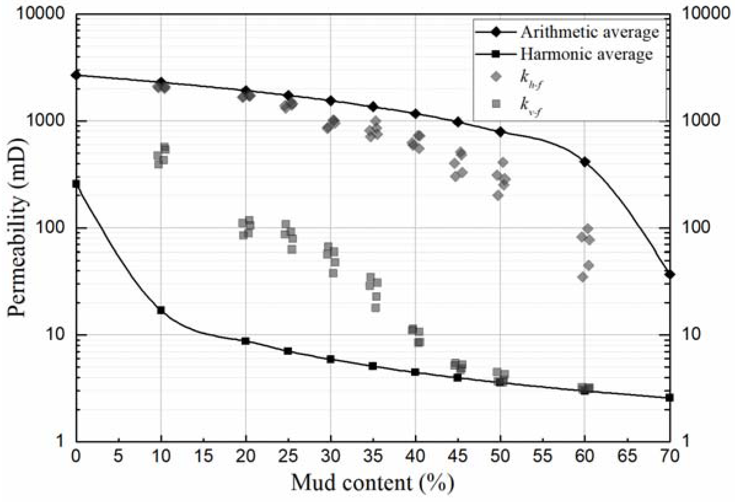
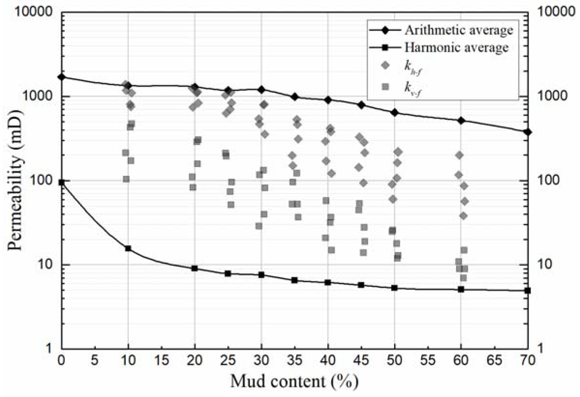
3.2. Representative Effective Permeability of the ISWZs

The k_v and k_h of individual realizations of each ISWZ calculated at full model size are respectively called the “k_v-f” and “k_h-f” in this article. All the k_v (circles) and k_h (diamonds) for all ninety realizations are shown in Figure 13 and Figure 14.

It is clearly observed that permeability values can span up to two orders of magnitude for all realizations, which indicates that the permeability calculated at the full model size is highly correlated with the mud content of an ISWZ. Note that the largest size of an ISWZ is not always its V_s, especially for ISWZs with varying width, which denotes that the V_s does not always exist. For all ISWZs, the k_v-f and k_h-f obviously follow a functional relationship with the ISWZ mud content (see Figure 13 and Figure 14). For ISWZs with constant width, k_h-f of an ISWZ linearly decreases as the mud content increases and is close to the upper solid line (the arithmetic average of the input permeability values of the fillings) when mud is below 0.25; then it deviates from this line and declines rapidly. However, the trend for k_v-f is different from that of k_h-f; although permeability also decreases linearly with the increase in mud content, k_v-f have a larger slope compared to k_h-f and deviate from the lower solid line (the harmonic average) until mud > 0.45. This behavior is consistent with the percolation threshold theory which holds that permeability is related to the dominant component (gravel for k_h-f, mud for k_v-f) as gravel provides a main flow path across the ISWZ, but mud is a barrier. These results are different from the two-components system proposed by Nordahl et al. [41]. For ISWZs with variable width, there is a similar behavior for k_h-f when the mud content is below 0.25. However, the results are clearly different for k_v-f, which decreases linearly with the increase in mud content and deviates from the harmonic average all the time. We assume that the width change of an ISWZ may significantly increases its permeability heterogeneity degree.

It is obvious that the V_s for different ISWZs is significantly different, requiring various methods for calculation. Ringrose et al. [42] proposed flow upscaling regimes to determine the V_s in a two-component heterogeneous porous medium. Nordahl et al. [41] extended their findings, which are different from some observations obtained by this study. Here, a series of three components of highly heterogeneous ISWZs considering variable width are developed and the results above further extend their findings.

Table 5. The calculation results of V_s for all the studied ISWZs.

ISWZ Type		Vs (m)
		For Horizontal Direction	For Vertical Direction
Constant width (100 cm)	Type1 (mud = 0.1)	<0.5	3
	Type2 (mud = 0.2)	<0.5	2.5
	Type3 (mud = 0.25)	<0.5	3.5
	Type4 (mud = 0.3)	<0.5	2.5
	Type5 (mud = 0.35)	<0.5	1
	Type6 (mud = 0.4)	<0.5	<0.5
	Type7 (mud = 0.45)	<0.5	<0.5
	Type8 (mud = 0.5)	2.5	<0.5
	Type9 (mud = 0.6)	N/A	<0.5
Varying width (10–100 cm)	Type10 (mud = 0.1)	40	N/A
	Type11 (mud = 0.2)	65	N/A
	Type12 (mud = 0.25)	75	N/A
	Type13 (mud = 0.3)	70	N/A
	Type14 (mud = 0.35)	N/A	N/A
	Type15 (mud = 0.4)	N/A	N/A
	Type16 (mud = 0.45)	N/A	N/A
	Type17 (mud = 0.5)	N/A	60
	Type18 (mud = 0.6)	N/A	65

gives the estimated results of V_s for all eighteen ISWZs, where the Cv values remain below 0.5 are regarded as valid. The V_s values of an ISWZ calculated in the vertical and horizontal directions are called the “V_s-v” and “V_s-h” in this article, respectively.

We find that the V_s values of ISWZs with constant width are one order of magnitude larger than those of ISWZs with constant width. For ISWZs with constant width, the V_s-v can be found in most ISWZs. However, the absence of the V_s-h occurs when mud >0.55. For ISWZs with varying width, the V_s for most of them cannot be found for either horizontal direction or vertical direction, and this behavior occurs for V_s-v and V_s-h when mud <0.5 and >0.3, respectively. Although the calculated V_s data are scarce, several trends can be clearly seen from the ISWZs with constant width: V_s-v decreases linearly to a mud share of 0.35; after the V_s-v declines rapidly and closes to the size of about 0.5 m. For V_s-h, a similar relationship can be observed, although it is not obvious. In addition, note that V_s-h and V_s-v cannot be found when mud >35 and <45, respectively. For ISWZs with varying width, it is not clear whether the V_s is beyond the full model size or indeed does not exist; further work to confirm this hypothesis is needed.

In this article, strictly speaking, k_s of an ISWZ exist only when its V_s can be found. However, for ISWZs with varying width, V_s cannot be found in most ISWZs. Considering that each ISWZ will attempt to determine the only k_s, here we regard the arithmetic mean permeability between the five realizations computed at the full model size as a good approximation of k_s of an ISWZ since the permeability variability at the full model size is the smallest among all scales. The k_s values of an ISWZ calculated in the vertical and horizontal directions are called the “k_s-v” and “k_s-h” in this article, respectively.

Table 6. The calculation results of k_s for all the studied ISWZs.

ISWZ Type		ks (mD)
		For Horizontal Direction	For Vertical Direction
Constant width (100 cm)	Type1 (mud = 0.1)	2074.8	482
	Type2 (mud = 0.2)	1707.4	101.6
	Type3 (mud = 0.25)	1416.6	85.8
	Type4 (mud = 0.3)	941.8	54
	Type5 (mud = 0.35)	826	27.2
	Type6 (mud = 0.4)	645.2	10.4
	Type7 (mud = 0.45)	405.4	5.12
	Type8 (mud = 0.5)	291.8	3.98
	Type9 (mud = 0.6)	81	3.178
Varying width (10–100 cm)	Type10 (mud = 0.1)	1044	378.8
	Type11 (mud = 0.2)	1072	199.2
	Type12 (mud = 0.25)	834.8	126
	Type13 (mud = 0.3)	584	94.6
	Type14 (mud = 0.35)	330.4	72.4
	Type15 (mud = 0.4)	270.2	32.6
	Type16 (mud = 0.45)	232.8	34.2
	Type17 (mud = 0.5)	154.2	19.8
	Type18 (mud = 0.6)	105.6	13.2

gives the calculated k_s for all eighteen ISWZs.

The comparison between the traditional permeability and the calculated k_s, shown in Figure 15, also reveals that all the calculated k_s go between the harmonic averages and arithmetic averages on the one hand, and a monotonic decrease with the mud content on the other hand.

The k_s-h values of ISWZs with constant width are always greater than those of ISWZs with varying width. However, the opposite conclusion can be drawn for k_s-v. Based on the above results, a few rules have been discovered to confirm k_s of an ISWZ. First, the effective continuum media theory will be the most suitable method for estimating k_s of an ISWZ when its V_s follows a linear trend with a relatively low mud fraction. Secondly, for ISWZs for which the content of mud is close to the percolation threshold, where the effective continuum media theory breaks down, a percolation threshold theory would be ideal for determining k_s. Thirdly, for ISWZs that behave as a stratified medium, the traditional average of permeability gives the best estimation for k_s (arithmetic average and harmonic average for k_s-h and k_s-v, respectively).

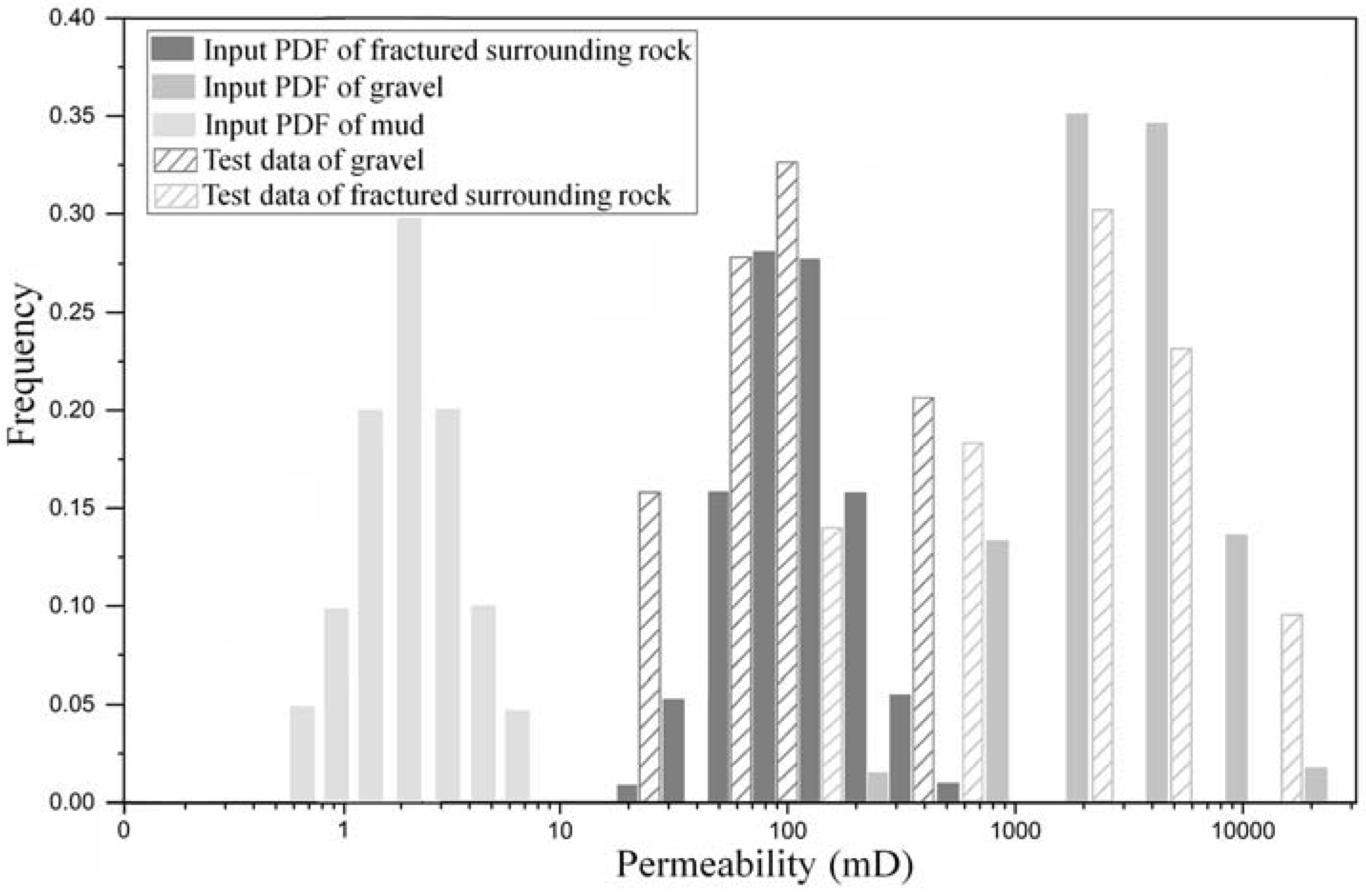
3.3. Verification of The Proposed Numerical Model

In order to validate the proposed numerical models of ISWZs, their predictions were utilized to compare with the field-test results of the permeability of C₃ which is one of the ISWZs developed on both sides of the Baihetan mountains (see Figure 1). The permeability data of C3 are all derived from the water-pressure tests in 30 boreholes (see

Table 7. Field-test results of permeability for C₃.

Test Method	Number	k (mD)	Sample Number	k (mD)	Sample Number	k (mD)
Water-pressure test by Hohai University (boost)	No. 1	11.5	No. 2	213.3	No. 3	825.7
Water-pressure test by Hohai University (depressurization)	No. 4	328.7	No. 5	222.6	No. 6	365.1
Laboratory test	No. 7	108.2	No. 8	149.8	No. 9	24.9
Water-pressure test by ECIDI	No. 10	32.4	No. 11	317.6	No. 12	70.3
	No. 13	17.6	No. 14	625.7	No. 15	175.8
	No. 16	574.4	No. 17	912.3	No. 18	912.3
	No. 19	10.1	No. 20	736.5	No. 21	617.6
	No. 22	116.5	No. 23	211.8	No. 24	133.8
	No. 25	29.7	No. 26	39.2	No. 27	623.2
	No. 28	1154.8	No. 29	458.7	No. 30	1287.3

). Field scanline surveys for C₃ (data collected more than 140-m-long outcrop) indicate the minimum, maximum, mean and standard deviation of width are, respectively, 14 cm, 108 cm, 44 cm and 15.6 (see Table 2), and its mud, gravel and fractured surrounding rock content are 8.3, 30.2 and 61.5, respectively. One point worth noting is that the permeability data obtained from our water-pressure tests can only represent the horizontal permeability estimated for a small-scale ISWZ whose size is about 4 m.

This point implies we cannot utilize these permeability data to describe the k_s of C₃; the test data can only represent the permeability of the test region. As shown in Figure 16, all field-test data are within the predicted permeability domain, which suggests that the proposed method and numerical ISWZs are valid and realistic. Additionally, the V_s of C₃ have not found, and the predicted k_s-h and k_s-v are 1012.4 mD and 96.4 mD, respectively.

This modeling method does also have some shortcomings. Although there is an acceptable match between the actual ISWZ and the numerical ISWZ, the former has a greater variability than the latter, and the results shown in Figure 16 just verify this statement. That is partly because it is impossible to include all fine-scale geometry and permeability information into numerical models and partly because the permeability input data of the fillings are only approximate descriptions of their fine-scale permeability information since our samples from three types of the fillings are not enough to cover all their permeability uncertainty and variability. In addition, the permeability data obtained by laboratory test are usually overestimated, especially for permeability that is a hydrogeological parameter with high variability. Despite these constraints, the procedures adopted in this article are regarded as acceptable since the generated numerical models have captured the most important geometry features that influence their flow properties.

4. Discussion

The ISWZs simulated in this article quantitatively indicate that the hydraulic behavior of a structural plane cannot simply be classified into two end-members. For example, an ISWZ usually acts as a conduit for fluid flow parallel to it, while it is a barrier for flow perpendicular to it. The strong positive influence of high-permeability gravel on the horizontal permeability, in addition to the negative impact of low-permeability mud on the vertical permeability, illustrates the significance of a precise description of the local structure. The SGS and SIS adopted in this article are both geostatistical algorithms. The modelling results for all ISWZs indicate that geometry models generated by SIS are adequate to describe the small-scale geometry features that influence flow properties. The permeability model developed by SGS differs from the traditional hydrogeological model which generally regards the permeability of any medium as a fixed value. The SGS was adopted in this article to develop permeability models, allowing the permeability values of each filling to have a non-fixed value but is constrained by a log-normal distribution.

Although this study uses a relatively small number of samples, commenting on the variability in the permeability of an ISWZ (k_h and k_v) as a function of sample scale is still useful. Results indicate that, for all ISWZs, the variation of permeability decreases with an increase in sample scale. However, the permeability value usually displays an upward trend. When comparing different types of ISWZs, it is observed that the scale effect on horizontal permeability shows a minimum, whereas the vertical permeability displays the highest variation at the lowest mud content considered (10%). Furthermore, for ISWZs with a constant width, both horizontal and vertical permeabilities display greater variation for ISWZs with changing width. In conclusion, the width distribution and filling content are the main factors affecting the permeability properties of an ISWZ.

At the scale where permeability is not sensitive to small variations in size, local homogeneity can be assumed [39] instead of identifying a representative effective permeability (k_s) and the size of a statistically homogeneous region (V_s) for each realization. The variability of permeability between the five realizations (Cv) is used to quantify the variation at any sample size between the five realizations. When Cv remains below 0.5 (a homogeneous range), k_s and V_s can be found, which is more reliable than the use of one realization. In general, the trend of Cv has a negative linear gradient as scale increases as expected. However, the calculation results of Cv in this article demonstrate that the Cv always fluctuates with increasing scale for some ISWZs. It is assumed that this abnormal trend is due to the lack of realizations for these ISWZs. Further work, that incorporates more realizations, may identify a more precise definition of flow properties of ISWZs.

In practice, even for the same structural plane, the field-test results may show up to 1–2 orders of magnitude difference in the permeability values (see Table 7). This arises from the difficulty in selecting appropriate values for the hydrogeological parameters of any ISWZ. Based on the findings of the research, some limits for the value of the permeability for ISWZs are proposed for the analyzing of groundwater flow problems in hydraulic engineering. These limits can be noted as follows: When studying the reservoir leakage and groundwater flow in mountains during reservoir filling, the values of permeability of the ISWZ should be chosen within the range of several meters to several tens of meters because ISWZs usually running through the entire project area. Furthermore, the seepage deformation problems of ISWZs exposed on the slope or underground chambers and the permeability values of an ISWZ should be selected within the range from centimeter to meters due to it relationship with the particle size of the fillings. For problems pertaining to slope stability caused by an ISWZ, the permeability values of an ISWZ should be defined based on the range of the slope failure.

Large-scale permeability characteristics of ISWZs are mainly controlled by fine-scale geometry and permeability features. Therefore, more detailed geometry and permeability information in ISWZs is best to provide a more comprehensive understanding of their seepage effect on groundwater flow in the subsurface. Our calculations are also helpful in giving insight into the permeability characteristics of ISWZs and as a way to identify the main controls (e.g., mud, gravel and fractured surrounding rock) on groundwater flow in an ISWZ. Once these controls are clearly established for a particular type of ISWZs, proper correlations between the permeability properties and a few measurable geometry parameters (e.g., the filling content) can be established. The procedure introduced here for identifying permeability of an ISWZ could be applied to ISWZs of any type, assuming a detailed geometry and permeability characterizations are available. Additionally, though some types of ISWZs that represent a range of mud contents are studied in this paper, only two extreme cases of wide distribution are modelled. More types of ISWZs should be conducted in future studies, including ISWZs which represent a range of width distributions.

5. Conclusions

The following main conclusions can be drawn.

• A set of eighteen realistic numerical models of ISWZs were developed by geostatistical modeling, each with five stochastic realizations. The models represent common ISWZs that have variable effective permeability on their horizontal and vertical axes and on different scales. Additionally, the permeability variation displays a downward trend as the sample scale increases for all types of ISWZs.
• The width distributions and filling content are the main factors affecting the permeability properties of an ISWZ. The ISWZ that has a higher mud content will lead to a larger scale effect on ISWZ horizontal permeability, while the opposite is true for its vertical permeability. Furthermore, the ISWZs with changing width would have greater permeability variation than that of ISWZs with constant width.
• The permeability variation between the five realizations at each scale step is expressed by the Cv. When Cv remains below 0.5, this can be used as an indication that local homogeneity has been achieved at a particular sample scale (V_s). The estimated V_s varies as a function of ISWZ type, and varies for horizontal and vertical permeability.
• The modeling and simulation methods introduced here could be adopted to other types of ISWZs and can be applied to develop accurate relationships for ISWZ permeability as a function of sample scale and other ISWZ petrophysical parameters.

References

1. Singhal, B.B.S.; Gupta, R.P. Applied Hydrogeology of Fractured Rocks; Springer Science & Business Media: Dordrecht, The Netherlands, 2010; pp. 13–33. [Google Scholar]
2. Gurocak, Z.; Alemdag, S. Assessment of permeability and injection depth at the Atasu dam site (Turkey) based on experimental and numerical analyses. Bull. Eng. Geol. Environ. 2012, 71, 221–229. [Google Scholar] [CrossRef]
3. Berhane, G.; Walraevens, K. Geological challenges in constructing the proposed Geba dam site, northern Ethiopia. Bull. Eng. Geol. Environ. 2013, 72, 339–352. [Google Scholar] [CrossRef]
4. Yano, T.; Aoki, K.; Ohnishi, Y.; Ohtsu, H.; Nishiyama, S.; Takagi, K. Methodology for estimation of the strength of rock discontinuities by using shearing tests under constant normal stiffness condition. Proc. JSCE 2010, 729, 115–130. [Google Scholar] [CrossRef]
5. Xu, D.P.; Feng, X.T.; Cui, Y.J.; Jiang, Q. Use of the equivalent continuum approach to model the behavior of a rock mass containing an interlayer shear weakness zone in an underground cavern excavation. Tunn. Undergr. Space Technol. 2015, 47, 35–51. [Google Scholar] [CrossRef]
6. Cui, Z.; Sheng, Q.; Leng, X. Control Effect of a Large Geological Discontinuity on the Seismic Response and Stability of Underground Rock Caverns: A Case Study of the Baihetan #1 Surge Chamber. Rock Mech. Rock Eng. 2016, 49, 2099–2114. [Google Scholar]
7. Shi, C.P.; Feng, X.T.; Jiang, Q.; Xu, D.P. Preliminary study of microstructural properties and chemical modifications of interlayer shear weakness zone in Baihetan. Rock Soil Mech. 2013, 34, 1287–1292. [Google Scholar]
8. Mancktelow, N.S.; Pennacchioni, G. The control of precursor brittle fracture and fluid–rock interaction on the development of single and paired ductile shear zones. J. Struct. Geol. 2005, 27, 645–661. [Google Scholar] [CrossRef]
9. Caine, J.S.; Evans, J.P.; Forster, C.B. Fault zone architecture and permeability structure. Geol. Soc. Am. 1996, 24, 1025–1028. [Google Scholar] [CrossRef]
10. Cleary, P.W.; Pereira, G.G.; Lemiale, V.; Piane, C.D.; Clennell, M.B. Multiscale model for predicting shear zone structure and permeability in deforming rock. Comput. Part. Mech. 2016, 3, 179–199. [Google Scholar] [CrossRef]
11. Jourde, H.; Flodin, E.A.; Aydin, A.; Durlofsky, L.J.; Wen, X.H. Computing permeability of fault zones in eolian sandstone from outcrop measurements. AAPG Bull. 2002, 86, 1187–1200. [Google Scholar]
12. Sibson, R.H. Structural permeability of fluid-driven fault-fracture meshes. J. Struct. Geol. 1996, 18, 1031–1042. [Google Scholar] [CrossRef]
13. Fisher, Q.J.; Knipe, R.J. The permeability of faults within siliciclastic petroleum reservoirs of the North Sea and Norwegian Continental Shelf. Mar. Pet. Geol. 2001, 18, 1063–1081. [Google Scholar] [CrossRef]
14. Evans, J.P.; Forster, C.B.; Goddard, J.V. Permeability of fault-related rocks, and implications for hydraulic structure of fault zones. J. Struct. Geol. 1997, 19, 1393–1404. [Google Scholar] [CrossRef]
15. Zhang, Z.; Li, X.; He, J. Numerical Study on the Permeability of the Hydraulic-Stimulated Fracture Network in Naturally-Fractured Shale Gas Reservoirs. Water 2016, 8, 393. [Google Scholar] [CrossRef]
16. He, Y.; Cheng, S.; Rui, Z.; Qin, J.; Fu, L.; Shi, J.; Wang, Y.; Li, D.; Patil, S.; Yu, H. An improved rate-transient analysis model of multi-fractured horizontal wells with non-uniform hydraulic fracture properties. Energies 2018, 11, 393. [Google Scholar] [CrossRef]
17. Baiocchi, A.; Dragoni, W.; Lotti, F.; Piacentini, S.M.; Piscopo, V. A multi-scale approach in hydraulic characterization of a metamorphic aquifer; what can be inferred about the groundwater abstraction possibilities. Water 2015, 7, 4638–4656. [Google Scholar] [CrossRef]
18. Bonnet, E.; Bour, O.; Odling, N.E.; Davy, P.; Main, I.; Cowie, P.; Berkowitz, B. Scaling of fracture systems in geological media. Rev. Geophys. 2001, 39, 347–383. [Google Scholar] [CrossRef] [Green Version]
19. Figueiredo, B.; Tsang, C.F.; Rutqvist, J.; Niemi, A. A study of changes in deep fractured rock permeability due to coupled hydro-mechanical effects. Int. J. Rock Mech. Min. Sci. 2015, 79, 70–85. [Google Scholar] [CrossRef] [Green Version]
20. Jiang, X.W.; Wang, X.S.; Wan, L. Semi-empirical equations for the systematic decrease in permeability with depth in porous and fractured media. Hydrogeol. J. 2010, 18, 839–850. [Google Scholar] [CrossRef]
21. Sanford, W.E. Estimating regional-scale permeability–depth relations in a fractured-rock terrain using groundwater-flow model calibration. Hydrogeol. J. 2017, 25, 405–419. [Google Scholar] [CrossRef]
22. Maryška, J.; Severýn, O.; Vohralík, M. Numerical simulation of fracture flow with a mixed-hybrid FEM stochastic discrete fracture network model. Comput. Geosci. 2005, 8, 217–234. [Google Scholar] [CrossRef]
23. Malkovsky, V.I.; Pek, A.A. Influence of an unconnected fracture system on the average permeability of rocks for a regular corridor pattern of isolated cracks. Petrology 2005, 13, 187–192. [Google Scholar]
24. Hanor, J.S.; Chamberlain, E.L.; Tsai, F.T. In evolution of the permeability architecture of the baton rouge fault zone, louisiana gulf coastal plain. In Proceedings of the AGU Fall Meeting 2011, San Francisco, CA, USA, 5–9 December 2011. [Google Scholar]
25. Shipton, Z.K.; Soden, A.M.; Kirkpatrick, J.D.; Bright, A.M.; Lunn, R.J. How Thick Is a Fault? Fault Displacement-Thcikness Scaling Revisited; American Geophysical Union (AGU): Washington, DC, USA, 2006; pp. 193–198. [Google Scholar]
26. Fourno, A.; Grenier, C.; Benabderrahmane, A.; Delay, F. A continuum voxel approach to model flow in 3D fault networks: A new way to obtain up-scaled hydraulic conductivity tensors of grid cells. J. Hydrol. 2013, 493, 68–80. [Google Scholar] [CrossRef] [Green Version]
27. Deutsch, C.V. A sequential indicator simulation program for categorical variables with point and block data: BlockSIS. Comput. Geosci. 2006, 32, 1669–1681. [Google Scholar] [CrossRef]
28. Juang, K.W.; Chen, Y.S.; Lee, D.Y. Using sequential indicator simulation to assess the uncertainty of delineating heavy-metal contaminated soils. Environ. Pollut. 2004, 127, 229–238. [Google Scholar] [CrossRef] [PubMed]
29. Lee, S.Y.; Carle, S.F.; Fogg, G.E. Geologic heterogeneity and a comparison of two geostatistical models: Sequential Gaussian and transition probability-based geostatistical simulation. Adv. Water Resour. 2007, 30, 1914–1932. [Google Scholar] [CrossRef]
30. Mayer, J.M.; Stead, D.; Bruyn, I.D.; Nowak, M. A sequential gaussian simulation approach to modelling rock mass heterogeneity. In Proceedings of the 48th U.S. Rock Mechanics/Geomechanics Symposium, Minneapolis, MN, USA, 1–4 June 2014; American Rock Mechanics Association: Alexandria, VA, USA, 2014. [Google Scholar]
31. Hicks, P.J. Unconditional sequential Gaussian simulation for 3-D flow in a heterogeneous core. J. Pet. Sci. Eng. 1996, 16, 209–219. [Google Scholar] [CrossRef]
32. Verly, G. Sequential Gaussian Simulation: A Monte Carlo Method for Generating Models of Porosity and Permeability; Springer: Berlin/Heidelberg, Germany, 1993; pp. 345–356. [Google Scholar]
33. Journel, A.G. Geostatistics: Models and tools for the earth sciences. Math. Geol. 1986, 18, 119–140. [Google Scholar] [CrossRef]
34. Jiang, X. The Study of Permeability of Basalts and Its Shear Zone. Geotech. Investig. Surv. 2008, 44, 25–26. [Google Scholar]
35. Zhang, R.; Jiang, Z.; Sun, Q.; Zhu, S. The relationship between the deformation mechanism and permeability on brittle rock. Nat. Hazards 2013, 66, 1179–1187. [Google Scholar] [CrossRef]
36. Espada, M.; Muralha, J.; Lemos, J.V.; Jiang, Q.; Feng, X.T.; Fan, Q.; Fan, Y. Safety Analysis of the Left Bank Excavation Slopes of Baihetan Arch Dam Foundation Using a Discrete Element Model. Rock Mech. Rock Eng. 2018, 3, 1–19. [Google Scholar] [CrossRef]
37. Yu, Y.; Wang, E.; Zhong, J.; Liu, X.; Li, P.; Shi, M.; Zhang, Z. Stability analysis of abutment slopes based on long-term monitoring and numerical simulation. Eng. Geol. 2014, 183, 159–169. [Google Scholar] [CrossRef]
38. Freeze, R.A. A stochastic-conceptual analysis of one-dimensional groundwater flow in nonuniform homogeneous media. Water Resour. Res. 1975, 11, 725–741. [Google Scholar] [CrossRef]
39. Corbett, P.W.M.; Jensen, J.L. Estimating the mean permeability: How many measurements do you need. First Break 1992, 10, 89–94. [Google Scholar] [CrossRef]
40. Jensen, J.; Lake, L.W.; Corbett, P.; Goggin, D. Statistics for Petroleum Engineers and Geoscientists, 2nd ed.; Handbook of Petroleum Exploration and Production 2 (HPEP); Elsevier Science: New York, NY, USA, 2000. [Google Scholar]
41. Nordahl, K.; Ringrose, P.; Wen, R. Petrophysical variation as a function of scale and implications for core-log integration. In Proceedings of the 65th EAGE Conference & Exhibition, Stavanger, Norway, 2–5 June 2003. [Google Scholar]
42. Ringrose, P.; Nordahl, K.; Wen, R. Vertical permeability estimation in heterolithic tidal deltaic sandstones. Pet. Geosci. 2005, 11, 29–36. [Google Scholar] [CrossRef]
Figure 1. Several maps of the Baihetan dam site. (a) Geographical location map; (b) Geological section map; (c) Distribution diagram for the main structural planes; (d) Simplified diagram of spatial distribution of some main hydrogeological structures.
Water 10 00779 g001
Figure 2. Massive rock containing an ISWZ (C3) which is located at the right bank of the Baihetan dam site area with the buried depth of about 500 m: (a) The picture of C3 taken at the scene; (b) The corresponding structure diagram.
Water 10 00779 g002
Figure 3. Grain size distribution curve of the fillings (grains from the interlayer soil of ISWZs, which are developed on both sides of the mountains of the Baihetan dam site).
Water 10 00779 g003
Figure 4. One realization of the numerical model of an ISWZ at the 40 m scale with a mud share of 30%. (a) The geometric model with three components represent mud (red), gravel (blue) and fractured surrounding rock (yellow), respectively; (b) The corresponding permeability model. The model size in (a,b) is 40 × 40 m.
Water 10 00779 g004
Figure 5. Comparison between the permeability input information and the measured permeability data.
Water 10 00779 g005
Figure 6. Sketch illustrating the sub-samples with different scales regularly extracted from a realization.
Water 10 00779 g006
Figure 7. How the horizontal permeability (kh) varies with the increase in sample size for ISWZs with constant width. Each solid line is the result of one of the realizations for a certain ISWZ type, and the dotted line represents the Cv value calculated from the five realizations at each scale step.
Water 10 00779 g007
Figure 8. How the vertical permeability (kv) varies with the increase in sample size for ISWZs with constant width.
Water 10 00779 g008
Figure 9. How the horizontal permeability (kh) varies with the increase in sample size for ISWZs with varying width.
Water 10 00779 g009
Figure 10. How the vertical permeability (kv) varies with the increase in sample size for ISWZs with varying width.
Water 10 00779 g010
Figure 11. Cv curves for ISWZs with constant width: vertical permeability (right) and horizontal permeability (left).
Water 10 00779 g011
Figure 12. Cv curves for ISWZs with varying width: vertical permeability (right) and horizontal permeability (left).
Water 10 00779 g012
Figure 13. Permeability calculation results of each realization at the full model size (for ISWZs with constant width-10 m). The lines represent the harmonic and arithmetic means of the input permeability values of the fillings.
Water 10 00779 g013
Figure 14. Permeability calculation results of each realization at the full model size (for ISWZs with varying width-100 m).
Water 10 00779 g014
Figure 15. ks calculation results for all eighteen ISWZs.
Water 10 00779 g015
Figure 16. Comparison between the calculated permeability of C3 and its field-test results (the ISWZ scale is about 4 m): horizontal permeability (left) and vertical permeability (right).
Water 10 00779 g016