Nonstationary Multivariate Hydrological Frequency Analysis in the Upper Zhanghe River Basin, China


1
State Key Laboratory of Hydrology-Water Resources and Hydraulic Engineering, Hohai University, Nanjing 210098, China
2
College of Hydrology and water resources, Hohai University, Nanjing 210098, China
*
Authors to whom correspondence should be addressed.
Water 2018, 10(6), 772; https://doi.org/10.3390/w10060772
Submission received: 16 May 2018
/
Revised: 8 June 2018
/
Accepted: 11 June 2018
/
Published: 12 June 2018
(This article belongs to the Section Hydrology)
Abstract
:Design annual runoff is a classical issue in traditional univariate hydrological frequency analysis (HFA). We developed a multivariate HFA approach for designs for a study region covering the confluence of two streams. HFA relies on the assumption that probability distribution is consistent in the past, present, and future; however, it has been asserted as incorrect under an uncertain and changing environment. A change-point was detected in our study and adopted to divide runoff into two periods, with no significant trends in all subseries. The post-change design annual runoff witnessed dramatic mean value decline by about half at four frequencies (50%, 75%, 90% and 95%), which were selected in the bivariate analysis. Probability distribution models were constructed with univariate p-III distributions through Clayton, Frank, and Gumbel copulas and independence. Frank copula showed a generally better match with observations than others. The traditional approach, adding up the same-frequency results from both tributaries independently, was disproved by the systematically smaller design values in independence model than copulas and the 40% asynchronous encounter probability. The 25.6% worst synchronous dry-dry encounter situation may be a concern for water resource managers. Consequently, multivariate HFA should prevail as design approach in terms of water resources security.
1. Introduction
The north part of China is under high water stress and suffers from physical water scarcity [1]. This area experiences not only all three leading factors for severe water scarcity nationwide (less water and unevenly distributed; rapid development and urbanization with a large and increasing population; poor water resource management) [2], but also has remarkable agriculture production with low precipitation in the growing season when crops are highly dependent on irrigation. Yang et al. [3] pointed out that water scarcity is an increasing constraint to the development of agricultural production in northern China, and a pricing mechanism is recommended to deal with the intensifying irrigated water stress under current water management institutions. The case study of the Upper Zhanghe River Basin in this region, exemplifies many existing conflicts (e.g., water scarcity, fuzzy boundaries, irrigated agriculture, environmental pollution, economic development and dense population, etc.) and poor water management intensifies the threat. Effective and practical government regulation is expected to challenge water issues, and economic related policies should be adopted to improve water management [4]. The implementation of Most Stringent Water Resources Management in China [5] reflects a growing attention of the government, and the clarification of Initial Water Rights is the foundation and prerequisite for the successful execution. Water resources assessment is the essential basis for optimal water resources allocation as well as initial water rights allocations, considering the randomness of the hydrological phenomenon, which is mainly approached through runoff sequence HFA. This paper provided an improvement to the traditional approach, to further offer reliable data support for the Initial Water Rights allocation.
Traditional HFA shows two major shortcomings. For one thing, hydrological sequences are assumed to be independent identically distributed (I.I.D.) random samples. More generally, the probability distribution of certain hydrologic random variable (e.g., annual runoff) is considered constant, thus, its characteristic parameters can be obtained through observed series. In other words, hydrological sequence is supposed to be consistent and its distribution is calculable. However, in the environment where transforming rainfall into runoff has been changed mainly due to climate variability and human activities, the hydrologic variables may not be independently and identically distributed [6]. This challenges the theoretical basis of traditional analysis and makes its reliability suspected, along with its application in hydraulic engineering. Therefore, testing nonstationarity and analyzing its influence on the design values are necessary prerequisites to HFA. Additionally, traditional HFA approaches are commonly studied in a univariate context. However, there are different dimensional sources in extreme and encounter events in many water-related issues that need probabilistic modelling. Hydrological extremes have multi-specific features, such as extreme floods having peak volume and maximum volumes in different durations, and extreme rainstorms having intensity, capacity and duration. While various participants consist in the synchronous-asynchronous encounter events, for instance, rainfall and runoff usually form wetness-dryness encounters in inter-basin water allocation; and local flood encounters in design flood region composition. Instead of focusing on each of these sources separately through univariate distribution in classical methods, recent multivariate HFA approaches considered them jointly to take into account their dependence structure. Chebana et al. [7] proposed a new framework for HFA using the hydrographs as one infinite-dimensional observation, and provided more effective and efficient estimates of the risk associated with extreme flood events by fully employing all the information contained in the hydrographs. Favre et al. [8] used copulas to model multivariate extreme values and applied the methodology to two different problems in hydrology: combined risk of peak flows in the framework of HFA, and joint modeling of peak flows and volumes. Despite of a wide variety of useful bivariate models to choose from, copula is flourishing in hydrology for its flexibility and applicability, which models dependent variables regardless of distribution while still able to capture nonlinear dependence structure between them [9]. In this study, the joint probability distribution of two tributaries annual runoff in the Upper Zhanghe River Basin is discussed though the promising method of 2-D copulas.
Multivariate studies are prone to ignore checking assumptions before modelling. In a univariate framework, HFA relies on consistency assumption that probability distribution is consistent in the past and future, thus, the future distribution can be deduced from the past, and in a multivariate framework, the joint distribution would be assumed to be the sum of single streams at same frequencies. Therefore, traditional HFA research mistakenly focused on spurious single populations, under an ungrounded independent assumption. To overcome the fundamental deficiency of the traditional method, in this study, the observed annual runoff data were first restored to nature runoff, and then the representative data was applied to test the stationarity assumption, to analyze the change-points and monotonic trends, and to uncover the root cause of nonstationarity and its contribution to design annual runoff. Moreover, copula was adopted in joint probability distribution modelling, in order to analyze the probability of wetness-dryness encounters of two tributaries supplying water to the region, and more generally, to give support to the optimal initial allocation of water resources in the Upper Zhanghe River Basin.
2. Materials
2.1. Study Area
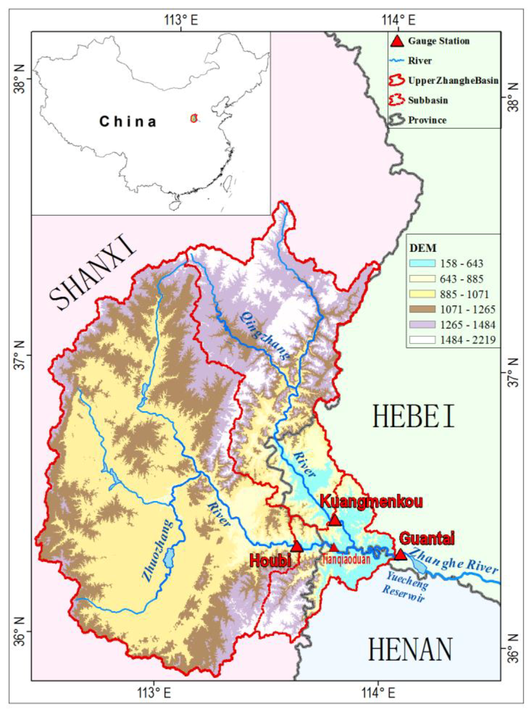
The Zhanghe River, a major tributary of the South Grand Canal in the Haihe River Basin, originates in Shanxi province and flows eastward through the administrative boundaries along Hebei and Henan provinces. The Upper Zhanghe River Basin refers to the region above the Yuecheng Reservoir’s Guantai Section, controls drainage area of 17,800 km2, stretching between longitudes 112.44–114.06° E and latitudes 35.86–37.60° N, where mostly mountainous terrain with intermontane Shangdang Basin exists (Figure 1). The river system is arranged in a fan, thick branching pattern, flowing across the Taihang Mountains, with steep mountains, overlapping peaks and sparse vegetation on both sides. Only few river terrace and flood land is left as subsistence farmland resources for local residents along the river (around 133 to 200 m2/capita). At the beginning of this centenary, this region has 4.188 million population (mostly farmer); many reservoirs and irrigated districts; and a rapid industrial growth, with insufficient irrigation water (about 400 m3/capita/year) and a high industrial and agricultural output value ratio (4.29 in 2000), therefore water resources are in great demand; however, deficient and unevenly distributed in time and space. The regional annual mean precipitation is about 570.4 mm, approximately 73% of which concentrates in one or two heavy rains at late July or early August. Hence, the natural stream flow distribution disaccords with agricultural water demand, while the irrigation season is April-to-June and November, when are low water months. There are two main tributaries in the Upper Zhanghe River Basin, Zhuozhang River and Qingzhang River, each mainly gauged by one hydrological station at downstream section, the Houbi station (Shanxi) controls 11,206 km2 area of Zhuozhang River Basin and the Kuangmenkou station (Hebei) 4159 km2 area of Qingzhang River Basin. The Zhanghe River Upstream Authority manages the whole region through the Houbi-Kuangmenkou-Guantai Reach (HKGR in the paper), to be more exact, from the Houbi and Kuangmenkou sections on tributaries to Guantai section of mainstream. The HKGR is the major water resources consumption of the Upper Zhanghe River Basin, as the water source for 49 villages in three provinces, containing four big irrigation canals, the Red Flag Canal, Yuejin Canal, Dayuefeng Canal, and Xiaoyuefeng Canal. Complicated natural environmental conditions, severe water scarcity, upstream-downstream shared rivers and ever-growing large population drive the region into one of the most prominent areas with frequent water-related disputes and conflicts nationwide.
2.2. Data and Restoring Calculation
Daily precipitation datasets of ten national meteorological stations were collected for the period 1956 to 2017. The series length of each station was varied due to the continuous updating of national meteorological system, among which only three cover most of the study time horizon, with 61 years of data (1957–2017). Annual runoff data was gathered for the same period from two hydrological gauge stations (Houbi and Kuangmenkou) situated near the outlets of the main two sub-basins. The runoff data at Guantai section was not collected, in that its value is roughly equal to the sum of the volume at two upstream sections, for no inflow over the small interval area of HKGR, and not essential in the analysis. The collection of runoff data also included the annual runoff sequence of Tianqiaoduan station and division volumes from four canals (Red Flag Canal, Tianqiaoyuan Canal, Baishanyidao Canal and Xida Canal), among which first three are located in the Zhuozhang River Basin and one in the Qingzhang River Basin.
Due to the under-representation of natural flow, restoring calculation is prerequisite in the analysis. For the Zhuozhang River, the Houbi station operates since 1995 so that extension of dataset is required. Tianqiaoduan station is located not far downstream Houbi section and controls similar drainage area of 11,250 km2, with longer complete observation records since 1956. There are three canals between two stations along the Zhuozhang River, whose diversion volumes were added up to the observed series at Tianqiaoduan section, to extend and restore the natural runoff at Houbi section. While for the Qingzhang River, the Xida power station, established in 1991, diverts streamflow upstream the Kuangmenkou section to generate electricity and drainages downstream in considered time horizon. The measured water amount of the Xida diversion canal was recovered to the dataset from the Kuangmenkou station.
3. Methods
3.1. Statistic Detection Tests
To date, many researchers have developed various effective tests to detect abrupt change [10,11,12] and monotonic trends [13,14,15]. In this study, non-parametric tests were adopted to detect change-points and trends, for being less subject to outliers, thus more suitable for dealing with skewness data in HFA. To be more precise, step changes in the population of mean annual runoff were tested by Moving Rank Sum test and Pettitt test, and monotonic trends of subpopulations were detected using Spearman Rank Correlation test and Mann-Kendall test [16].
3.1.1. Abrupt Change Detection Tests
Moving rank sum (MRS) test and Pettitt test were applied to check the stationarity assumption in the study. In general, both are non-parametric tests derived from Mann–Whitney U test for whether two samples come from the same population in a similar way, introducing a test statistic whose extreme value indicates the existence of step change, under certain conditions. Observations are probed through a sliding pointer in chronological order, among which the special one points out the change-point according to the location of the extreme.
The MRS test is a rank-based test with a statistic U, approximate normal distribution with significance level α,
where n1 is the size of smaller population and n2 the other, according to the sliding pointer τ, and W is the sum of ranks for smaller size sample. If the maximum absolute value of U (|U|max) > Uα/2, then the ‘change’ hypothesis will be accepted, whose corresponding time is the change-point.
Pettitt test’s statistic Ut,n,
where n is the length of the series, and . At the special sliding pointer t0, let |Ut,n|max be k0, if ≤ 0.5, then the stationarity hypothesis will be rejected, and the corresponding time of t0 is the change-point [17].
3.1.2. Monotonic Trend Detection Tests
Spearman rank correlation (SRC) test and Mann-Kendall (MK) test were employed in trends detection. Both are non-parametric rank-based tests, evaluating the relationship between chronological order and value of series through a test statistic.
The statistic of SRC test follows Student’s t-distribution with degrees of freedom v = n − 2 and significance level α. The ‘no trend’ hypothesis will not be rejected if |tSRC| < tv,α/2.
where n is the length of series, rSRC (Spearman rank correlation coefficient) is calculated by , di = Ri − i, i represents the chronological order, Ri the rank.
The MK [18,19] test statistic , where n is the length of the series, xi, xj are data and sgn ( ) is a sign function . For n ≥ 10, S is approximate normal distribution, and its standardized form Z is
The ‘no trend’ hypothesis will not be rejected if |Z| < Zα/2.
3.2. Hydrological Frequency Analysis Methods
3.2.1. p-III Distribution
Many hydrological variables are better characterized by Pearson type III (p-III), a three-parameter Gamma distribution, frequently used for volumes [20]. The PDF (probability density function) of the standard p-III distribution is expressed as
where α, β and ε are respectively the shape, scale and location parameters. These parameters can be identified by the expected value (μ), standard deviation (σ), and coefficient of skewness (γ) of the distribution through the equations: ; ; [21]. Various methods have been developed to estimate the three parameters in the hydrological frequency calculation, such as Probability Weighted Moments Method, Weighted Function Method [22] and L-Moments Method [23]. L-moments method was applied in this study.
3.2.2. Copulas
A copula is a function that links the same amount of marginal distributions to form a multivariate distribution function, which offers a possibility to model the dependence structure independently of the marginal distributions. Assuming that two random variables (X and Y) are related, Sklar’s [24] theorem states that if FX,Y (x,y) is a bivariate distribution function with marginal cumulative distribution functions FX (x) and FY (y), a copula C can be denoted as
Archimedean Copula is more popular in practical applications because of its clear structure, simple computation and high adaptability. In a bivariate distribution case, a copula C could be called Archimedean Copula if it admits the expression , where ϕ (u) is the generator function, a continuous, strictly decreasing and convex function such that ϕ (0) = ∞, ϕ(1) = 0; ϕ−1 is its pseudo-inverse function such that ϕ−1(∞) = 0, ϕ−1(0) = 1 [25]. Most common Archimedean copulas are Gumbel Copula, Frank Copula, Clayton Copula, etc., based on their generators (Table 1). All these three copula types have been considered in this research.
4. Results and Discussion
4.1. Stationarity Test
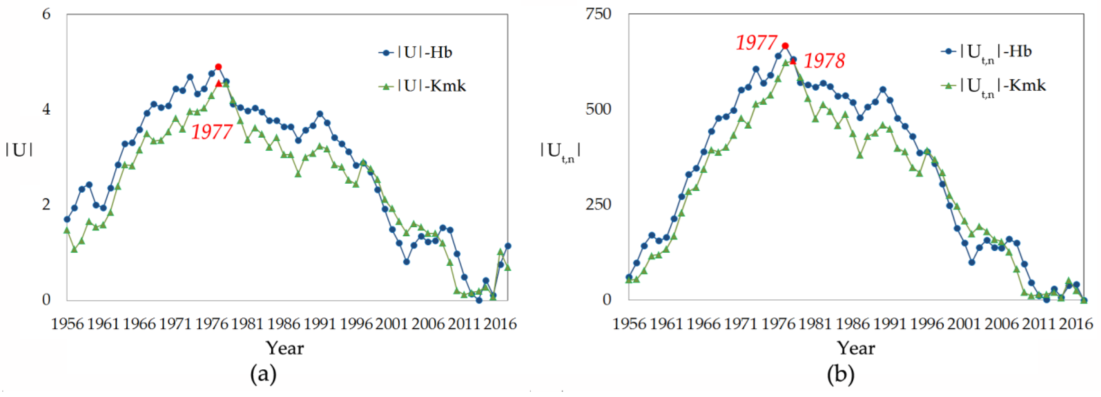
Stationarity assumption was checked by non-parametric tests before modelling. For the whole study period from 1956 to 2017, the annual runoff series of both tributaries change with tendency, and the sudden change in mean value was accepted in 1978 as concluded by the MRS test and the Pettitt test. Both test statistics showed the extreme value in 1977 at Houbi section, which could be taken as valid, because the |U|max (4.90) was larger than 1.96 in the MRS test and (3.38 × 10⁻⁵) was less than 0.5 in the Pettitt test. While even though the valid results of two tests were different at Kuangmenkou section, both test statistics appeared similar values in 1977 and 1978, the difference is less than 0.22% (0.01 out of 4.56 (|U|max)) in MRS test, and 0.80% (5 out of 627 (|Ut,n|max)) in Pettitt test, whose were 1.18 × 10⁻⁴. Therefore, the population may consider varies since 1978, the research time horizon was partitioned into two sub-periods, pre-change (1956–1977) and post-change (1978–2017) periods. The test statistics of the two methods are shown in Figure 2.
All subseries passed stationarity test with no significant monotonic trends detected in the SRC test and the MK test. The significance level α was selected as 0.05 in both tests. While for the SRC test, the threshold was determined also by a parameter related with data size, which was 20 and 38 for two sub-periods, so the t20,0.05/2 and t38,0.05/2 represent the critical value for the pre- and post-period separately, in Table 2.
Observed streamflow in most of rivers in Northern China experiences the decreasing trend, affected by the changes of climate and land surface environment [27], these two factors were considered responsible for the abrupt change and dramatic decrease in runoff series and will be mainly discussed below.
4.2. Runoff Decline Reason Analysis
The annual runoff shows downtrend and the decrement is calculated between subseries. The mean annual runoff of Zhuozhang River decreases 548 million m3 (from 984 to 437), while for Qingzhang River the value is 286 million m3 (from 550 to 264). Runoff is extremely sensitive to precipitation, secondly to that is rainfall-runoff relationship, thus the reason of runoff decreasing was discussed from these aspects. Stated another way, climate change and human activities are commonly considered as two major factors influence runoff trends, precipitation as the most sensitive climate factor to runoff, its variation implies the climate contribution; and its relationship with streamflow reflects the underlying surface conditions, which are the most striking effects from human activities.
4.2.1. Precipitation Variation
Annual regional rainfall and their sub-periods averages were calculated by Thiessen polygon method. The mean value of regional rainfall decreased 75.3 mm (from 598.8 to 523.5) in the Zhuozhang River Basin upstream Houbi section, and 71.9 mm (from 588.4 to 516.5) in the Qingzhang River Basin upstream Kuangmenkou section. Coherent trends with runoff were detected in precipitation, which suggested that the variation of precipitation upstream might be the main origin of the runoff changes.
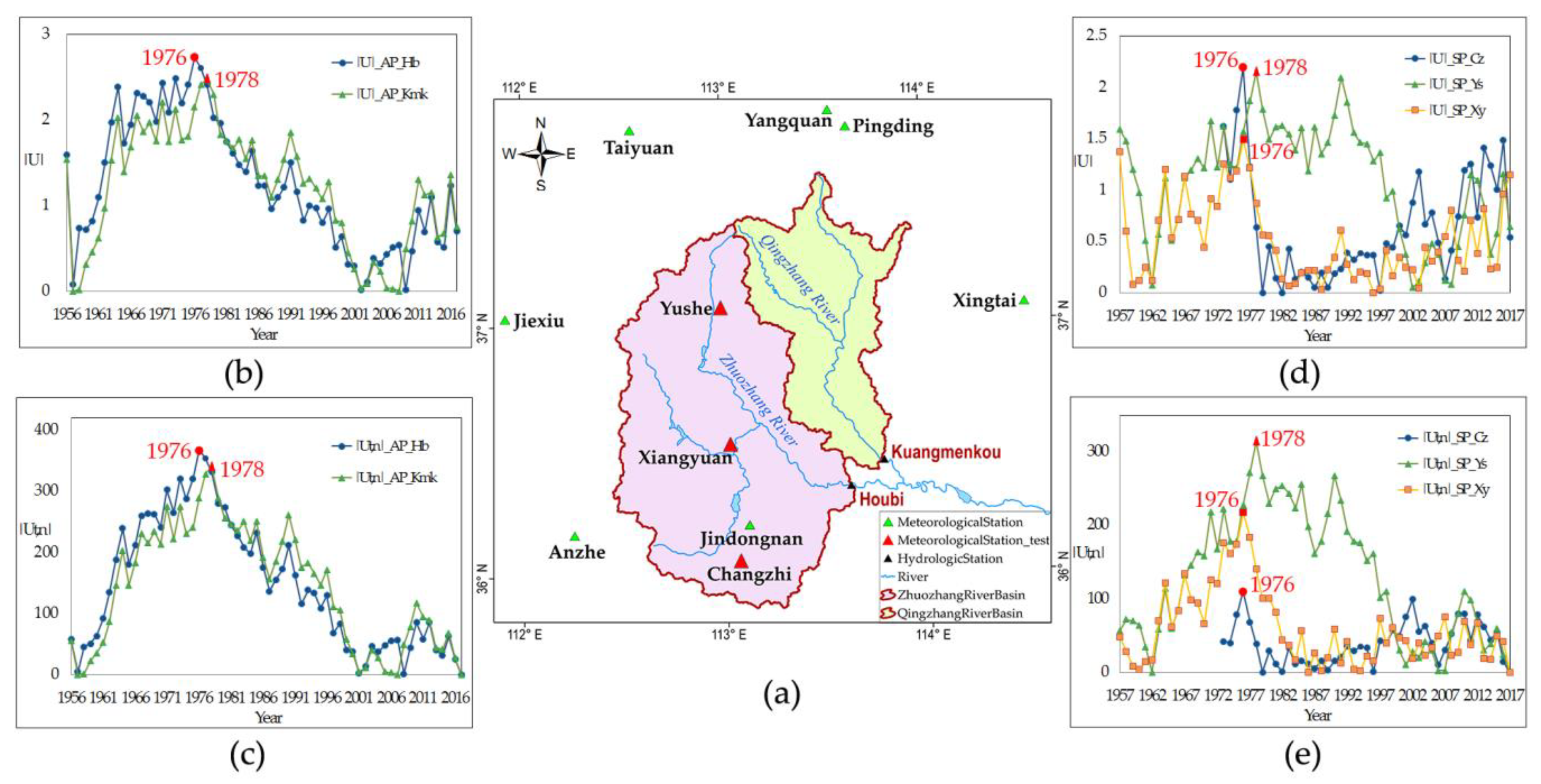
The annual areal precipitation (1956–2017) of two sub-basins were analyzed by MRS test and Pettitt test, abrupt points at 1976 for the Zhuozhang River basin and 1978 for the Qingzhang River basin were detected (Figure 3b,c), which were in coordination with the results of runoff. For Qingzhang River basin, the runoff displayed changing in 1977 and 1978, and the area rainfall reached the abrupt point almost simultaneously at the later year, which is reasonable for its relative small basin area, but still insufficient to explain the changing started previously, therefore, except for precipitation, other reasons should be concerned. As for the Zhuozhang River basin, it took precipitation more time to influence the runoff at Houbi section, due to its uneven distribution in the large area, so that three stations inside the basin with long time series were tested in the same way. The results showed that the rainfall around the west and south source (Xiangyuan and Changzhi) varied earlier at 1976 than the north source (Yushe) at 1978 (Figure 3d,e). Given that the Xiangyuan and Changzhi stations control larger area of the basin and nearer to the outlet, it’s more consistent with the whole Zhuozhang River basin in precipitation, thus their station precipitation directly reflect the area rainfall variation. In conclusion, the trends of precipitation that appeared in accordance with runoff, should be taken as the main reason for its variation.
Precipitation decrease problem has drawn a lot of attention, and the meteorological reason was uncovered in some works. Wagan et al. [28] studied the variations of precipitation from eight weather stations in the Zhanghe River Basin during 1980–2010, within the time horizon after 1978, among which only three stations (Changzhi, Yangcheng, Yushe) showed insignificant negative trends in annual precipitation, all in our studying area. Cai et al. [29] analyzed the decline reason for precipitation in the Zhang-Wei-South Canal drainage area and some cities around, like Changzhi, Anyang, covering our studying area. Although no significant decrease trends were detected among the annual rainfall (1957–2006) at the eight meteorological stations, but all of which changed with tendency and the average decrease reached 83.2 mm in the previous 50 years. Cai discussed that the most sensitive climate factor, temperature, showed most visible change among all the factors in the analysis, which coincided with the global climate change trends; and the year of 1978 is the turning point, when the temperature rises and precipitation drops forwards, affected by the bigger climate system; furthermore, the long duration of the trends among climate factors implies that this region is becoming warm-dry. Cai’s results were proved by the conclusion in the National Assessment Report on Climate Change (The Ministry of Science and Technology of the People’s Republic of China). In conclusion, the global climate change is the leading factor for the precipitation variation, and the decrease trend would continue.
4.2.2. Rainfall-Runoff Relationship
The transformation of rainfall into runoff is complex, especially for generating and routing processes, which are closely related to underlying surface. Human activities have a direct bearing on land surface variation, and consequently affect rainfall-runoff relationship, that is to say, the rainfall with similar characteristics would generate varied runoff processes at disturbed areas [30]. In this study, runoff coefficient, a dimensionless coefficient describing the percentage of precipitation turned into runoff, was adopted to assess the influence of underlying surface variation on the runoff process. We calculated sub-periods average runoff depth and assist them with average rainfall correspondingly, to get mean annual runoff coefficient (Table 3). The approximately half value drop of the coefficient implies that, in general, a similar rainfall process would only generate around half the runoff volume before the abrupt change appears.
The sharp decrease in runoff coefficient revealed that the runoff process was greatly varied by intensified human activities in the last 30 years. The Zhanghe River Basin is a seriously disturbed area in the Zhang-Wei-South Canal region, where is universally modified with land utilization and irrigation works. Farmland accounts for over 50 percent of its catchment area growing winter wheat and corn. Streamflow is mostly manipulated by 246 large-, medium- and small-sized reservoirs, with a total storage capacity of 3.844 billion m3, controlling over 95 percent of the valley area, supplying 36 large-sized irrigation districts. A rapidly growing population and increasing industrial and agricultural water consumption boost water withdrawal. To make matters worse, among the supplies, most of the water (about 70% to 80%) goes to agriculture with high loss ratio, more evaporation and less drainage. In addition, groundwater overdraft and coal mining increases leakage loss of surface water, especially rivers, which result in a sharp surface runoff reduction. Zeng et al. [31] separated the effects of climate change and human activities on runoff in the Zhanghe River Basin, and indicated that the climate change contributes more than human activities on annual runoff changes, while the major factor was changeable at seasonal and monthly scales.
4.3. Probability Distribution Analysis
4.3.1. Marginal Probability Distribution
HFA relies on several assumptions in terms of dataset, especially independence, identity and stationarity, and four annual runoff subseries of two tributaries before and after 1978 were adopted through statistical testing. The probability distributions and design annual runoff at given frequencies were calculated and drawn in Table 4 and Figure 4, by the parameters of subseries. Results show that the design annual runoff at normal year (p = 50%), dry year (p = 75%) and extreme dry year (p = 90% or 95%) during the post-change period all were about half the previous. Considering the analysis that aims at guiding current and future water resources allocation, the subseries before 1978 was unsuitable in the study because of its low representativeness. Hence the univariate marginal distribution derived from the 1978–2017 runoff sequences was taken as the basis of bivariate joint probability distribution computation.
In China, the CDF (cumulative distribution function) generally is formed as F(x) = p (X ≥ x) where X is a random variable, in order to emphasize low water, which is different with the popular function F(x) = p (X ≤ x). HFA usually focuses on the low flow and extreme low flow design, for that water shortage is the key problem to settle in water resources planning and management.
4.3.2. Joint Probability Distribution
The volume at the confluence is the combination of the runoff from two upstream sections. The resulting runoff can be written as Z = X + Y, where X is the random variable representing the volume at Houbi section and Y at Kuangmenkou. The aim is to design annual runoff of HKGR taking into account the dependence between the volumes from two tributaries for water security. The bivariate distribution models were constructed with two univariate p-III probability distributions, and four types were considered: The independence, Clayton, Frank and Gumbel copulas. In our case, the formula (6) can be written as
,
with ~ p-III(1.38, 0.19, 2.66), ~ p-III(1.02, 0.28, 1.84) for pre-change period;
~ p-III(3.19, 0.89, 0.78), ~ p-III(0.84, 0.49, 0.92) for post-change period.
Positive dependence was detected by Kendall’s τ and Spearman’s ρ in Table 5. The empirical value, obtained from observations, displayed that the correlation decreased between the two tributaries. Based on the simple relationship between Kendall’s τ and Copula’s α, the copula-constructed joint distribution functions were identified. Then the τ and ρ values of copulas were estimated. Through the comparison of τ and ρ, Frank and Gumbel showed a good behavior in the 1956–1977 period, similar in magnitude of the observation estimation, and Frank showed an obvious better match in the more recent period.
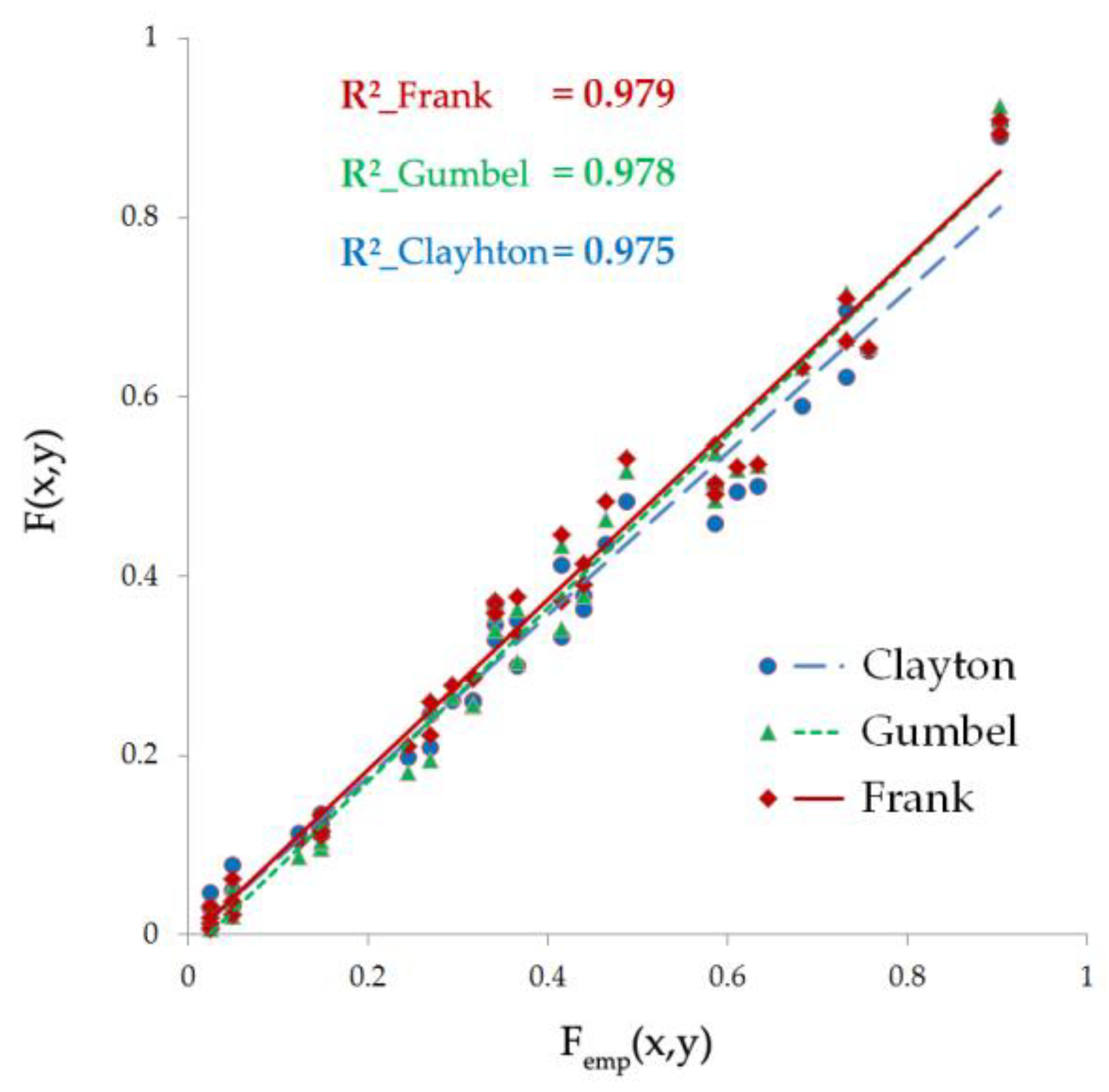
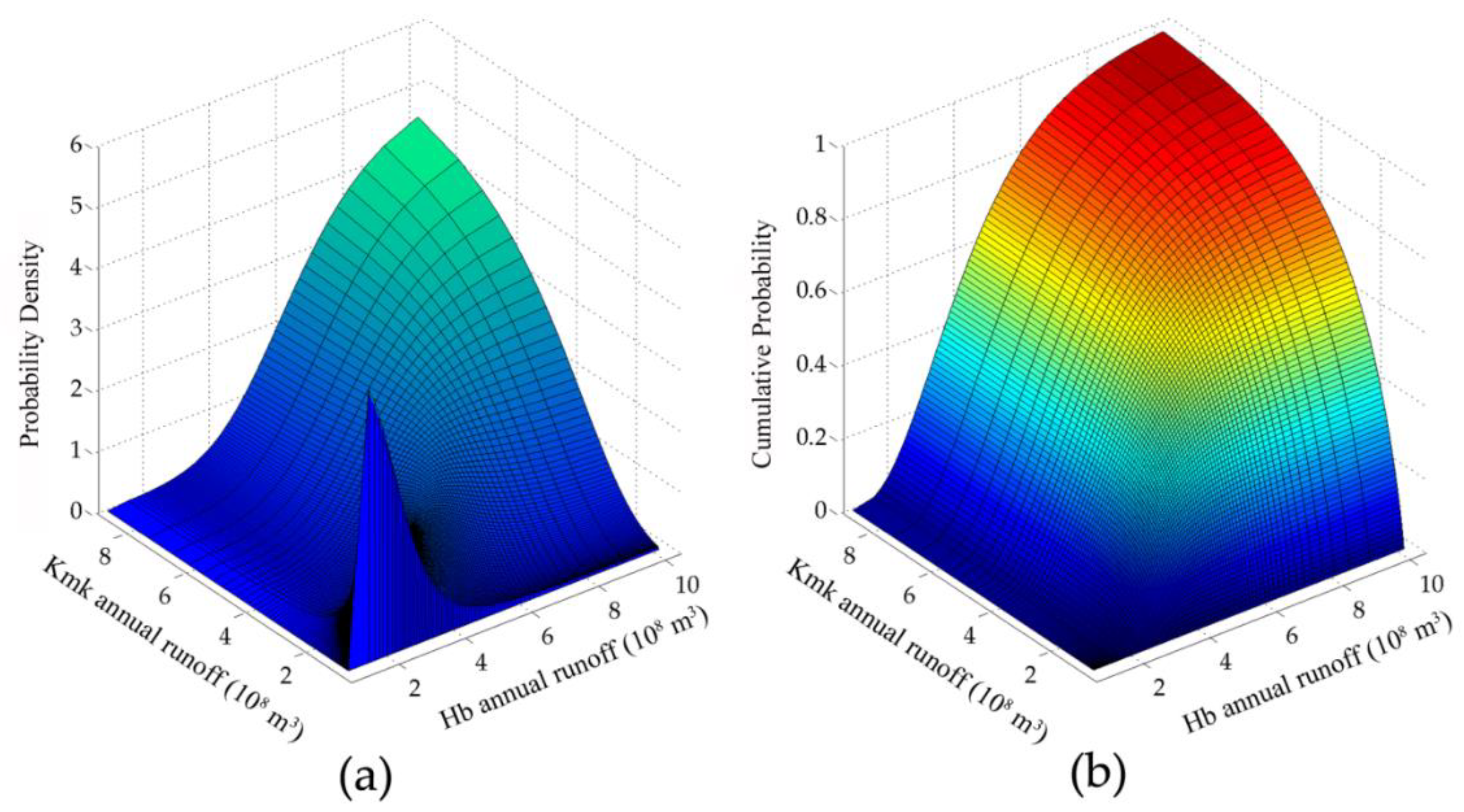
The effectiveness of copula-based theoretical distribution F(x,y) (FC, FF, and FG) were further analyzed, by the goodness-of-fit evaluation method, comparing with the empirical cumulative distribution Femp(x,y). As we proposed design runoff to guide future allocation, the period since 1978 was selected for its better representation. The correlation coefficient squares were all about 0.98, witnessed an overall good performance of the selected copulas, and Frank copula showed a slightly better behavior in Figure 5. Figure 6 illustrates the joint distribution in the case of Frank copula.
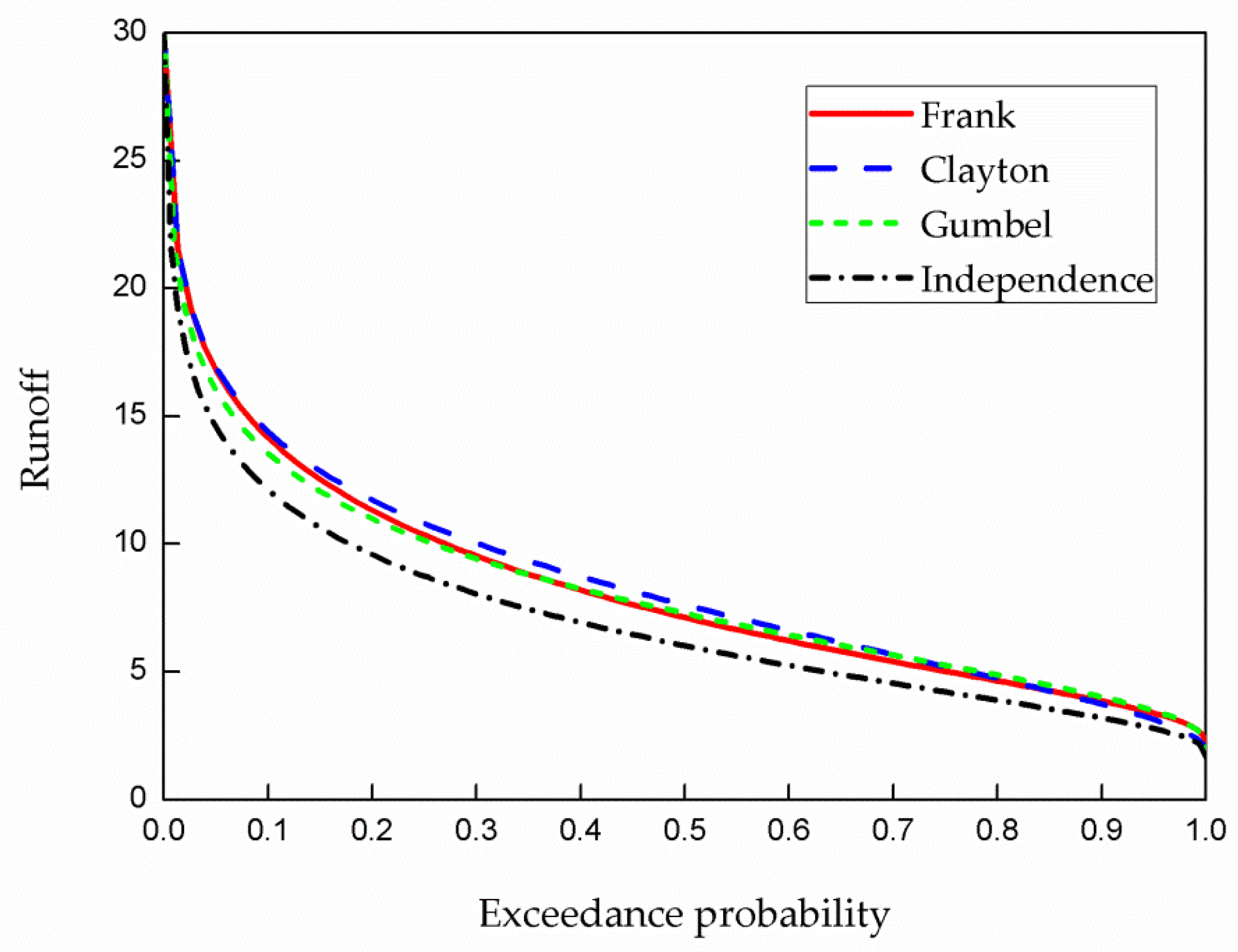
The cumulative distributions of copula-based models were calculated and plotted with the independence case in Figure 7. DFs in national HFA are commonly 50%, 75%, 90% and 95% on behalf of normal year (p = 50%), dry year (p = 75%), and extreme dry year (p = 90% or 95%). Interesting results are displayed in Table 6.
In general, minimal difference was shown from one copula to another, with the mean range within 4%, and Frank copula showed closest to the mean value of copulas. Clayton offered smallest value for extremely low flow (p ≥ 90%), and Frank gave the smallest for normal and low flow probabilities, and they shared the same mean value for the special DFs. Gumbel was not a good choice for targeted probabilities, because of its overall higher estimations. The independence gave systematically smaller quantile values than the three copulas, and the highest range was achieved for extremely low flow with a magnitude around 18%, furthermore, the mean range was about 17% for the interested DFs. The notable range between copulas and independence case directly falsified the I.I.D. assumption in traditional HFA, and proved that the series of tributaries were not independently distributed. Therefore, the neglect of dependence may lead to under-designing the annual runoff, and increasing hydrological risk.
Frank copula showed a generally better behavior in the tests above, covering the comparison with empirical distribution, independence case, and other copulas. Additionally, it is found to be the best-fitted one according to AIC (Akaike information criterion), which offered the smallest value of −0.13 comparing with −0.02 and 0 by Clayton and Gumbel respectively. Consequently the bivariate HFA approach was developed based on Frank copula in the study area. New method was applied to analyze the relationship between DFs of marginal distributions and the joint probabilities at the confluence. Events interested are shown in Table 7.
A few explanations help interpret the results in this section. First, the physical mechanisms for the joint frequency and the deviation from marginal were revealed through the bivariate distribution strategy. The independence case was a direct result of marginal distributions, the systematically smaller values in Table 6 uncovered that the deviation was an effect of dependence structure between tributaries. Furthermore, a positive correlation between the runoff of tributaries was also demonstrated by the Kendall’s τ and Pearson’s ρ of two epochs in Table 5, and the strong correlation displayed inadaptability to the current environments, since the value dropped from 0.62, 0.79 to 0.45, 0.65, respectively. The traditional approach works by adding up the marginal distributions at same frequency of all tributaries independently, which was disproved by the dependence between variables. In conclusion, although the traditional HFA prevails for its well application previously, the method has to be renewed due to an uncertain and changing environment. Second, some interpretation is needed for the design annual runoff at different DFs reported in Table 6. From a social perspective, DF is also known as assurance rate (AR) of water resources in water supply design, for its direct reflection of the assurance level. Water supply security is the real crisis facing the society, guaranteed rate instead of DF is the key target in engineering design, which is largely determined by the distribution of the water resources under certain frequency. Take an example in the table, in the previous studies, as the case of independence, the annual runoff reached 3.20 × 10⁸ m3 means the AR should be 90%, while copula offered even larger value at the frequency of 95% on 3.39 × 10⁸ m3, so at this magnitude of runoff it must take the pre-arranged planning for extremely low flow at 95% rather than the 90%’s, otherwise water deficits would appear due to under-designing. Third, the joint distribution was discussed above, and how it was connected to the marginal distributions was revealed in Table 7. For instance, runoff of both tributaries at 75% DF represents an event that two tributaries upstream witness two low flows encountering at the confluence, and their joint probability was calculated to be 64.40% by Frank copula, the slip told that the situation would happen more frequently than thought traditionally. In general, each type of dry situations is more likely to happen in HKGR than sub-basins. Then take one asynchronous encounter as example, DF at Houbi section is 50% and Kuangmenkou section is 95%, their joint probability is 49.58%. This is a normal-extreme dry encounter event, in which the major question would be whether it is a relief for the worse side. The results in this study only told us that the flow after merging slightly changed by the extreme dry tributary, thus the HKGR and Zhuozhang River still have normal runoff volume to supply, while about relieving the situation of Qingzhang River, engineering allocation should be taken into account.
4.4. Synchronous-Asynchronous Encounter Risk Analysis
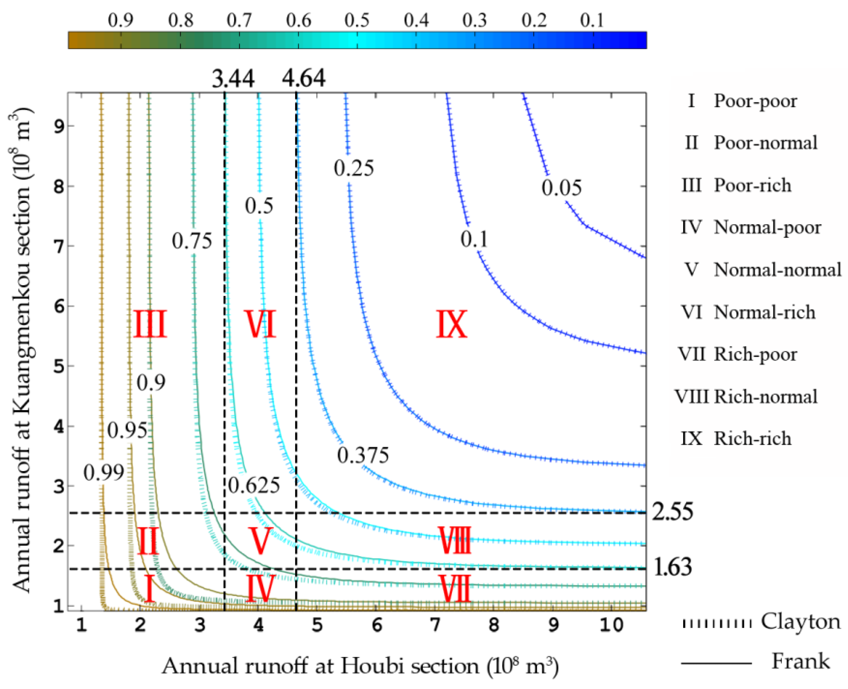
The encounter risk of runoff of main two tributaries was analyzed by the joint CDF , based on the frequency of 37.5% and 62.5%. 62.5% is the median of special probabilities for normal (50%) and low flow (75%); to guarantee that 50% still at the center of the normal flow range, the probability of 37.5% was selected reciprocally, between normal and high (25%) flow. The two probabilities were commonly adopted in encounter situation classification in China, for example, Zhang et al. [32]. Hence, the cumulative distribution p-III(x) ≤ 37.5% serves as wet year, 37.5% < p-III(x) ≤ 62.5% as normal year and p-III(x) > 62.5% as dry year, in a univariate setting. Then make the joint cumulative distribution be as synchronous wet year, as synchronous normal year and as synchronous dry year, called synchronous hydrological year, otherwise, it is asynchronous hydrological year for the region. In our case, the boundary values of marginal distributions were the design annual runoff 3.44 × 10⁸ m3(px = 62.5%), 4.64 × 10⁸ m3(px = 37.5%) at Houbi section (X) and 1.63 × 10⁸ m3(py = 62.5%), 2.55 × 10⁸ m3(py = 37.5%) at Kuangmenkou section (Y). The synchronous-asynchronous encounter situations of rich-poor annual runoff of tributaries could be classified as (with unit 108 m3): Rich-rich encounter probability: prr = P (X ≥ 4.64, Y ≥ 2.55); Rich-normal encounter probability: prn = P (X ≥ 4.64, 1.63 ≤ Y <2.55); Rich-poor encounter probability: prp = P (X ≥ 4.64, Y < 1.63); Normal-rich encounter probability: pnr = P (3.44 ≤ X < 4.64, Y ≥ 2.55); Normal-normal encounter probability: pnn = P (3.44 ≤ X < 4.64, 1.63 ≤ Y <2.55); Normal-poor encounter probability: pnp = P (3.44 ≤ X < 4.64, Y < 1.63); Poor-rich encounter probability: ppr = P (X < 3.44, Y ≥ 2.55); Poor-normal encounter probability: ppn = P (X < 3.44, 1.63 ≤ Y < 2.55); Poor-poor encounter probability: ppp = P (X < 3.44, Y <1.63). The Clayton copula offered an extreme option in bounding case, thus was also selected, to compare with Frank copula and research the sensitivity of the choices of copulas. The contour lines of the joint cumulative distribution for annual runoff of two tributaries and their encounter situations are displayed by Frank and Clayton copulas in Figure 8, and the results are in Table 8.
Make the joint probability be pxy for two tributaries, pxy_f for results by Frank and pxy_c by Clayton, in Figure 8. Frank copula agreed well with Clayton in wet year (pxy ≤ 37.5%), and the dot of Clayton started to leave Frank’s solid line ever since, especially for normal to extremely dry year (pxy ≥ 50%), where the runoff values of pxy_c were obviously smaller than that of pxy_f. Table 8 well illustrates the sensitivity of choices among copulas. We knew that Clayton offered smaller runoff estimations before this results, but did not have clear picture about the consequences. In this table, the two copulas obtained totally opposite conclusion about synchronous and asynchronous proportion. Through Frank copula, there is about 60% chance that the tributaries would have normal year or suffer from floods and droughts simultaneously, and over a quarter for each disaster situation; still 40% that one tributary would complement the other in need, which was ignored in the traditional HFA by assuming that tributaries share same DF. While this proportion reached 60% by Clayton copula, and the most desirable poor-rich encounter situation accounted for 11%, overwhelming the 3.7% by Frank, which would result in unprepared water shortage problems. Additionally, the worst synchronous poor-poor encounter risk given by Clayton was less than 17%, much smaller than it should be, comparing to 25.6% by Frank, and the authority may not pay enough attention to the situation on this basis. Therefore, the under-designing the probability of extreme runoff situation by Clayton copula could lead to severe water crisis in the study area, where is under high water stress and suffers from physical water scarcity.
We analyzed some special joint events in Table 7, and still want to know how likely different situations would happen, which is the encounter probability. The asynchronous encounter took a noticeable proportion in Table 8, accounted for 40%. Bivariate approach should be applied to solve the societal-scale challenge, since the dependence between runoff of tributaries should be taken into account. Another remarkable result is the 25.6% for dry-dry encounter risk, implying that the worst situation has a big chance to happen under the existing severe conditions. Correspondingly, dry-wet the most optimistic case of encounter only took 3.7%, so the prospects of complementing the other in need are very low. 60% synchronous encounter reflected a positive correlation between tributaries, which supported the results of correlation coefficients. It was the slip in the τ and ρ that told us that the strong positive correlation did exist but not last. The variation reason must lie in the hydrological processes, which are complicated, but the principal two factors that contribute most to runoff at outlets, are rainfall and underlying surface. We knew that the precipitation is changing with the climate system, and the human activist remodeled most of the region since 1950s. The global climate change drives the region into warm-dry, while the harm to the nature routing is discordant and haphazard, therefore both influences are extensive and unpredictable. In conclusion, the environment is uncertain and changing, and the study method should be renewed accordingly.
5. Conclusions
This study supplements the traditional frequency analysis method by pretesting nonstationarity of datasets and modelling bivariate distributions to address the questions arising from the assumptions in the commonly applied univariate approaches and to expand the existing framework of hydrological frequency analysis. The annual runoff sequences of two tributaries (Zhuozhang River and Qingzhang River) in the Upper Zhanghe River Basin were investigated to detect the abrupt changes and monotone trends in streamflow. The joint probability distribution for annual runoff of two tributaries was studied using the 2D-copula methods to discuss wetness-dryness encountering probabilities in the HKGR. The following conclusions have been reached in this study:
(1) Nonstationarity analyses showed that both the annual runoff sequences of two tributaries from 1956 to 2017 change with tendency, and the sudden change in mean value appeared in 1978. Univariate frequency analyses of all the subseries (before and after the change-point) revealed that the p-III distribution from two periods changed significantly, and the design values in the post-change period decreased into half the previous at all DFs (50%, 75%, 90% and 95%). Declining precipitation and frequent interference of human activities (reservoir construction, check dams and irrigation canals, groundwater exploitation, etc.) are considered responsible for the sharp decline in annual runoff, by hindering the generation and transportation of streamflow.
(2) The strong positive correlation before change-point was detected by Kendall’s τ and Pearson’s ρ, and the correlation displayed inadaptability to the new environments and the coefficients fell, thus the traditional HFA method should be improved. Through the comparison of the bivariate distribution models, Frank copula showed a generally better behavior, as it offered closest τ and ρ to the values obtained from observations and gained the highest correlation with the empirical cumulative distribution. It also displayed the smallest range to the mean of cumulative distributions among copulas. Meanwhile, the independence model estimated systematically smaller design values, so that the dependence structure is not neglectable, and the AR should be recalculated and upgraded according to the design values by Frank copula.
(3) In the encounter analysis, the probabilities slip at the synchronous situations from the tributaries to the confluence, implying that the dry situations are more likely to happen in HKGR than sub-basins. Asynchronous encounter took a noticeable 40%, uncovered that the runoff from tributaries were not identically distributed. In addition, the chance of most desirable dry-wet encounter only accounted for 3.7%, while the least expected dry-dry encounter risk, on the contrary, reached 25.6% in this severe water-shortage area. More attention should be paid and precautionary measures should be taken by water resource managers.
In summary, this study appropriately falsified the stationarity hypotheses in traditional frequency analysis approaches and it provided a more practical and suitable method under the current uncertain and changing environment. The developed strategy may lead to better estimates of design runoff, thus a more effective water resources assessment. Reliable, healthy, and convincing water rights allocation comes from the feasible, accurate and valid water assessment; therefore, this study offers scientific support for the water policy making and would be better for meeting the main interests of stakeholders in the near future.
Author Contributions
Conceptualization, G.L.; Data curation, H.G.; Formal analysis, G.L.; Funding acquisition, Z.Y. and G.L.; Investigation, H.G.; Methodology, G.L.; Project administration, Z.Y.; Resources, G.L. and Q.J.; Software, H.G.; Supervision, Z.Y.; Validation, Z.Y.; Visualization, H.G.; Writing—original draft, H.G. and G.L.; Writing—review & editing, H.G.
Acknowledgments
This work was supported by the National Key R&D Program of China (Grant No. 2016YFC0402710); National Natural Science Foundation of China (Grant No. 51479061, 51539003); National Science Funds for Creative Research Groups of China (No. 51421006); the program of Dual Innovative Research Team in Jiangsu Province and the Special Fund of State Key Laboratory of Hydrology-Water Resources and Hydraulic Engineering (Grant No. 20145027312); the project of Power Construction Corporation of China (Grant No. DJ-ZDZX-2016-02).
Conflicts of Interest
The authors declare no conflict of interest.
References
- Rijsberman, F.R. Water scarcity: Fact or fiction? Agric. Water Manag. 2006, 80, 5–22. [Google Scholar] [CrossRef] [Green Version]
- Jiang, Y. China’s water scarcity. J. Environ. Manag. 2009, 90, 3185–3196. [Google Scholar] [CrossRef] [PubMed]
- Yang, H.; Zhang, X.; Zehnder, A.J.B. Water scarcity, pricing mechanism and institutional reform in northern China irrigated agriculture. Agric. Water Manag. 2003, 61, 143–161. [Google Scholar] [CrossRef]
- Dosi, C.; Easter, K.W. Water scarcity: Institutional change, water markets and privatization. In Economic Studies on Food, Agriculture, and the Environment; Kluwer Academic: Plenum Bologna, Italy, 2002; pp. 91–115. [Google Scholar]
- Ge, M.; Wu, F.-P.; You, M. Initial provincial water rights dynamic projection pursuit allocation based on the most stringent water resources management: A case study of Taihu basin, China. Water 2017, 9, 35. [Google Scholar] [CrossRef]
- Milly, P.C.D.; Betancourt, J.; Falkenmark, M.; Hirsch, R.M.; Kundzewicz, Z.W.; Lettenmaier, D.P.; Stouffer, R.J. Stationarity is dead: Whither water management? Science 2008, 319, 573–574. [Google Scholar] [CrossRef] [PubMed]
- Chebana, F.; Dabo-Niang, S.; Ouarda, T.B.M.J. Exploratory functional flood frequency analysis and outlier detection. Water Resour. Res. 2012, 48, 4514. [Google Scholar] [CrossRef]
- Favre, A.-C.; El Adlouni, S.; Perreault, L.; Thiémonge, N.; Bobée, B. Multivariate hydrological frequency analysis using copulas. Water Resour. Res. 2004, 40. [Google Scholar] [CrossRef] [Green Version]
- Ashkar, F.; Aucoin, F. A broader look at bivariate distributions applicable in hydrology. J. Hydrol. 2011, 405, 451–461. [Google Scholar] [CrossRef]
- Jeon, J.-J.; Sung, J.H.; Chung, E.-S. Abrupt change point detection of annual maximum precipitation using fused lasso. J. Hydrol. 2016, 538, 831–841. [Google Scholar] [CrossRef]
- Buishand, T.A. Tests for detecting a shift in the mean of hydrological time series. J. Hydrol. 1984, 73, 51–69. [Google Scholar] [CrossRef]
- Reeves, J.; Chen, J.; Wang, X.L.; Lund, R.; Lu, Q. A review and comparison of changepoint detection techniques for climate data. J. Appl. Meteorol. Clim. 2007, 46, 900. [Google Scholar] [CrossRef]
- Haan, C.T. Statistical Methods in Hydrology; Iowa State University Press: Ames, IA, USA, 1977; p. 378. [Google Scholar]
- Kundzewicz, Z.W.; Robson, A.J. Change detection in hydrological records—A review of the methodology. Hydrol. Sci. J. 2004, 49, 7–20. [Google Scholar] [CrossRef]
- Chebana, F.; Ouarda, T.B.M.J.; Duong, T.C. Testing for multivariate trends in hydrologic frequency analysis. J. Hydrol. 2013, 486, 519–530. [Google Scholar] [CrossRef]
- Li, G.; Xiang, X.; Guo, C. Analysis of nonstationary change of annual maximum level records in the Yangtze river estuary. Adv. Meteorol. 2016, 2016, 1–14. [Google Scholar] [CrossRef]
- Pettitt, A.N. A non-parametric approach to the change-point problem. J. R. Stat. Soc. 1979, 28, 126–135. [Google Scholar] [CrossRef]
- Mann, H.B. Nonparametric tests against trend. Econometrica 1945, 13, 245–259. [Google Scholar] [CrossRef]
- Kendall, M.G. Rank Correlation Methods; Griffin: Oxford, UK, 1948; p. 108. ISBN 0-85264-199-0. [Google Scholar]
- Yue, S.; Ouarda, T.B.M.J.; Bobée, B. A review of bivariate gamma distributions for hydrological application. J. Hydrol. 2001, 246, 1–18. [Google Scholar] [CrossRef]
- Wu, Y.-C.; Liou, J.-J.; Su, Y.-F.; Cheng, K.-S. Establishing acceptance regions for l-moments-based goodness-of-fit tests for the Pearson type III distribution. Stoch. Environ. Res. Risk Assess. 2012, 26, 873–885. [Google Scholar] [CrossRef]
- Liang, Z.; Hu, Y.; Li, B.; Yu, Z. A modified weighted function method for parameter estimation of Pearson type three distribution. Water Resour. Res. 2014, 50, 3216–3228. [Google Scholar] [CrossRef] [Green Version]
- Hosking, J.R.M. L-moments analysis and estimation of distributions using linear combination of order statistics. J. R. Stat. Soc. 1990, 52, 105–124. [Google Scholar] [CrossRef]
- Sklar, M. Fonctions de répartition an dimensions et leurs marges. Publ. Inst. Statist. Univ. Paris 1959, 8, 229–231. [Google Scholar]
- Genest, C.; Rivest, L.P. Statistical inference procedures for bivariate Archimedean copulas. J. Am. Stat. Assoc. 1993, 88, 1034–1043. [Google Scholar] [CrossRef]
- Clayton, D.G. A model for association in bivariate life tables and its application in epidemiological studies of familial tendency in chronic disease incidence. Biometrika 1978, 65, 141–151. [Google Scholar] [CrossRef]
- Li, B.; Liang, Z.; Zhang, J.; Wang, G.; Zhao, W.; Zhang, H.; Wang, J.; Hu, Y. Attribution analysis of runoff decline in a semiarid region of the loess plateau, China. Theor. Appl. Climatol. 2016. [Google Scholar] [CrossRef]
- Wagan, B.; Hakimzadi, Z.A. Spatial and temporal variations of precipitation: Case study of Zhanghe River basin, P. R. China. J. Biodivers. Environ. Sci. 2015, 7, 76–86. [Google Scholar]
- Cai, X.; Zongxue, X.U.; Zhanling, L.I. Analyzing long-term trend of hydrological and meteorological changes in Zhangweinan River basin. Resour. Sci. 2008, 30, 363–370. [Google Scholar]
- Li, G.-F.; Xiang, X.-Y.; Tong, Y.-Y.; Wang, H.-M. Impact assessment of urbanization on flood risk in the Yangtze River delta. Stoch. Environ. Res. Risk Assess. 2013, 27, 1683–1693. [Google Scholar] [CrossRef]
- Zeng, S.; Xia, J.; Du, H. Separating the effects of climate change and human activities on runoff over different time scales in the Zhang River basin. Stoch. Environ. Res. Risk Assess. 2013, 28, 401–413. [Google Scholar] [CrossRef]
- Zhang, J.; Ding, Z.; You, J. The joint probability distribution of runoff and sediment and its change characteristics with multi-time scales. J. Hydrol. Hydromech. 2014, 62. [Google Scholar] [CrossRef]
Figure 1.
The Upper Zhanghe River Basin.

Figure 2.
Abrupt change detection for annual runoff series during 1956–2017 of two tributaries at Houbi (Hb) and Kuangmenkou (Kmk) sections, with maximum values of |U| in MRS test and |Ut,n| in Pettitt test both appearing in 1977 at Hb section, as for Kmk section, 1977 and 1978 showed similar extreme values in both tests, though with different results. (a) MRS test statistic |U|, based on formula (1); (b) Pettitt test statistic |Ut,n|, based on formula (2).

Figure 3.
Variation analysis of annual area and station precipitation. (a) National meteorological stations selected and their distribution, in green and red. All have contributed to annual area rainfall calculation for two sub-basins (b,c), and three in red were also tested to analyze trends in the Zhuozhang River basin (d,e); (b) MRS test (|U|) for area precipitation (1956–2017) of Houbi(|U|_AP_Hb) and Kuangmenkou(|U|_AP_Kmk); (c) Pettitt test (|Ut,n|) for area precipitation of two sub-basins during the same period; (d) MRS test for station precipitation of Changzhi (|U|_SP_Cz 1973–2017) at south source, Yushe (|U|_SP_Ys 1957–2017) at north source, and Xiangyuan (|U|_SP_Xy 1957–2017) at the merge of south and west source of the Zhuozhang River; (e) Pettitt test for station precipitation of three stations in different source regions in the Zhuozhang River basin.

Figure 4.
The univariate p-III distribution of annual runoff subseries of two tributaries during the pre-change and post-change periods. (a) Annual runoff distribution at Houbi (Hb) section; (b) Annual runoff distribution at Kuangmenkou (Kmk) section.
Figure 4.
The univariate p-III distribution of annual runoff subseries of two tributaries during the pre-change and post-change periods. (a) Annual runoff distribution at Houbi (Hb) section; (b) Annual runoff distribution at Kuangmenkou (Kmk) section.

Figure 5.
Empirical cumulative distribution Femp(x,y) versus theoretical cumulative distribution F(x,y) for the three types of copulas, Clayton, Frank, and Gumbel.
Figure 5.
Empirical cumulative distribution Femp(x,y) versus theoretical cumulative distribution F(x,y) for the three types of copulas, Clayton, Frank, and Gumbel.

Figure 6.
Joint distribution in the case of Frank copula. (a) Probability density distribution; (b) Cumulative probability distribution.
Figure 6.
Joint distribution in the case of Frank copula. (a) Probability density distribution; (b) Cumulative probability distribution.

Figure 7.
Cumulative exceedance probability curves in the cases of Independence, Clayton, Frank and Gumbel copulas.
Figure 7.
Cumulative exceedance probability curves in the cases of Independence, Clayton, Frank and Gumbel copulas.

Figure 8.
Joint cumulative exceedance probability curves in the cases of Clayton and Frank copulas for annual runoff of tributaries, and synchronous-asynchronous encounter probability of rich-poor annual runoff at Houbi and Kuangmenkou sections (9 districts represent different encounter situations separately, depend on two annual runoff values of each stream at frequencies of 37.5% and 62.5%). Each district amounts to the projected area of cumulative distributions.


Table 1.
Bivariate Archimedean copulas and their generators.
| Bivariate Copula | Generator ϕ(t) | Parameter | CDF 1 |
|---|---|---|---|
| Clayton [26] | t−α − 1 | α > 0 | |
| Frank | α ≠ 0 | ||
| Gumbel | (−ln t)α | α ≥ 1 |
1 CDF is the abbreviation for Cumulative Distribution Function.
Table 2.
Monotonic trend detection for annual runoff subseries during pre-change and post-change periods.
Table 2.
Monotonic trend detection for annual runoff subseries during pre-change and post-change periods.
| Station | SRC Test | MK Test | Result | |||||
|---|---|---|---|---|---|---|---|---|
| |tSRC|_pre 1 | t20,0.05/2 2 | |tSRC|_post | t38,0.05/2 | |Z|_pre | |Z|_post | Z0.05/2 3 | ||
| Houbi | 1.045 | 2.086 | 0.233 | 2.024 | 1.015 | 0.739 | 1.96 | no trend |
| Kuangmenkou | 0.013 | 0.665 | 0 | 0.676 | no trend | |||
1 _pre and _post represent pre-change and post-change subseries; 2 critical value tv,α/2; 3 critical value Zα/2.
Table 3.
The mean annual runoff coefficient of upstream basins of two stations.
| Stations | Runoff Depth/mm | Mean Annual Runoff Coefficient | ||||
|---|---|---|---|---|---|---|
| 1956–1977 | 1978–2017 | 1956–1977 | 1978–2017 | Decrease | Rate/% | |
| Houbi | 88.6 | 39.3 | 0.148 | 0.075 | 0.073 | 49.0 |
| Kuangmenkou | 110.5 | 53.0 | 0.188 | 0.103 | 0.085 | 45.4 |
Table 4.
The hydrological frequency analysis results of annual runoff subseries at two sections.
| Station | Period | Parameters | Design Annual Runoff at DF 1/108 m3 | |||||
|---|---|---|---|---|---|---|---|---|
| μ | σ | γ | p = 50% | p = 75% | p = 90% | p = 95% | ||
| Houbi | 1956–1977 | 9.84 | 0.62 | 1.70 | 8.21 | 5.41 | 3.92 | 3.41 |
| 1978–2017 | 4.37 | 0.46 | 1.12 | 4.00 | 2.89 | 2.15 | 1.81 | |
| Kuangmenkou | 1956–1977 | 5.50 | 0.66 | 1.98 | 4.39 | 2.91 | 2.23 | 2.03 |
| 1978–2017 | 2.64 | 0.71 | 2.18 | 2.03 | 1.33 | 1.05 | 0.98 | |
1 DF is the abbreviation for Design Frequency.
Table 5.
Comparison of rank correlation coefficient for copulas.
| Period | Type | Clayton | Frank | Gumbel | Empirical |
|---|---|---|---|---|---|
| 1956–1977 | Kendall | 0.4712 | 0.6248 | 0.5812 | 0.6190 |
| Spearman | 0.6496 | 0.8244 | 0.7695 | 0.7888 | |
| 1978–2017 | Kendall | 0.3474 | 0.4580 | 0.3927 | 0.4503 |
| Spearman | 0.4969 | 0.6450 | 0.5535 | 0.6546 |
Table 6.
Runoff of a given joint design frequency for tested models (108 m3).
| Exceedance Probability | Clayton | Frank | Gumbel | Independence |
|---|---|---|---|---|
| 95% | 3.14 | 3.39 | 3.49 | 2.79 |
| 90% | 3.74 | 3.87 | 4.03 | 3.20 |
| 75% | 5.22 | 5.02 | 5.27 | 4.22 |
| 50% | 7.62 | 7.13 | 7.28 | 6.03 |
Table 7.
The joint probabilities of annual runoff of two tributaries at given design frequencies by Frank copula (%).
Table 7.
The joint probabilities of annual runoff of two tributaries at given design frequencies by Frank copula (%).
| DF of Houbi Station | DF of Kuangmenkou Station | |||
|---|---|---|---|---|
| 50% | 75% | 90% | 95% | |
| 50% | 37.75 | 46.56 | 49.05 | 49.58 |
| 75% | 46.56 | 64.40 | 71.66 | 73.47 |
| 90% | 49.05 | 71.66 | 83.40 | 86.84 |
| 95% | 49.58 | 73.47 | 86.84 | 91.01 |
Table 8.
The frequency analysis of synchronous-asynchronous encounter of rich-poor annual runoff of tributaries in case of Frank and Clayton copulas (%).
Table 8.
The frequency analysis of synchronous-asynchronous encounter of rich-poor annual runoff of tributaries in case of Frank and Clayton copulas (%).
| Copula | Synchronous Frequency | Asynchronous Frequency 1 | |||||||||
|---|---|---|---|---|---|---|---|---|---|---|---|
| Poor-Poor | Normal-Normal | Rich-Rich | Total | Poor-Normal | Poor-Rich | Normal-Poor | Normal-Rich | Rich-Poor | Rich-Normal | Total | |
| Frank | 25.61 | 8.69 | 25.61 | 59.91 | 8.15 | 3.74 | 8.15 | 8.15 | 3.74 | 8.15 | 40.09 |
| Clayton | 16.98 | 6.38 | 16.98 | 40.34 | 9.31 | 11.21 | 9.31 | 9.31 | 11.21 | 9.31 | 59.66 |
1 Houbi v.s. Kuangmenkou.
© 2018 by the authors. Licensee MDPI, Basel, Switzerland. This article is an open access article distributed under the terms and conditions of the Creative Commons Attribution (CC BY) license (http://creativecommons.org/licenses/by/4.0/).
Share and Cite
MDPI and ACS Style
Gu, H.; Yu, Z.; Li, G.; Ju, Q. Nonstationary Multivariate Hydrological Frequency Analysis in the Upper Zhanghe River Basin, China. Water 2018, 10, 772. https://doi.org/10.3390/w10060772
AMA Style
Gu H, Yu Z, Li G, Ju Q. Nonstationary Multivariate Hydrological Frequency Analysis in the Upper Zhanghe River Basin, China. Water. 2018; 10(6):772. https://doi.org/10.3390/w10060772
Chicago/Turabian StyleGu, Henan, Zhongbo Yu, Guofang Li, and Qin Ju. 2018. "Nonstationary Multivariate Hydrological Frequency Analysis in the Upper Zhanghe River Basin, China" Water 10, no. 6: 772. https://doi.org/10.3390/w10060772
Note that from the first issue of 2016, this journal uses article numbers instead of page numbers. See further details here.