Statistical Distribution of TSS Event Loads from Small Urban Environments

Abstract

Results from a long-term stormwater quality monitoring program were used to derive total suspended solids (TSS) event load distributions at four small urban environments (flat roof, parking lot, residential catchment, high traffic street). Theoretical distribution functions were fitted to the empirical distribution functions obtained. Parameters of the theoretical distribution functions were optimized with respect to a likelihood function to get both optimized parameters and standard errors. Kolmogorov-Smirnov and Anderson-Darling test statistics were applied to assess the goodness-of-fit between empirical and theoretical distribution. The lognormal distribution function was found to be most expressive to approximate empirical TSS event load distributions at all sites. However, the goodness-of-fit of the statistical model strongly depends on the number of events available. Based on the results of a Monte-Carlo-based resampling strategy, around 40 events should be considered.

1. Introduction

The implementation of robust stormwater management strategies requires to address issues related to both water quantity and water quality [1]. Cost-effective measures are essential to protect the receiving ecosystem as much as required while still being resource-efficient. This expects an in-depth understanding of relevant stormwater processes. While hydrologic rainfall-runoff processes are well understood, stormwater quality processes are still focused by current research [2,3]. For example, continuous signals of UV-Vis spectrometers or turbidity sensors are frequently used to study intra-event pollutant processes and to estimate event loads or event mean concentrations [4,5,6,7,8]. The influence of environmental, temporal and spatial variables on intra-event dynamics and flushing characteristics of, e.g., the parameter total suspended solids (TSS) have been studied and analyzed by means of Mass–Volume–Curves [4,8,9,10]. Although the studies revealed site-specific tendencies in the proportion of washed-off load during storm events, the heterogeneous data presented clearly demonstrate the complex nature of pollutant processes, which is expressed by significant variability of pollutographs [8].

Pollutant generation from urban surfaces is generally due to two processes: the build-up and the wash-off [11]. Wash-off is known to be mainly driven by rainfall [12,13,14,15], surface type and use [16,17,18] and pollutant characteristics [13,17]. Recent developments have shown that physically-based wash-off models are outperforming long-existing conceptual models. For example, the authors in Reference [19] developed a saltation-type washoff model from laboratory experiments. Being mainly adapted from soil erosion research, the model detaches particles proportional to rainfall intensity and masses available at surface. Reference [20] modelled the wash-off process of a small road near Paris using a model system coupling the shallow water equations for overland flow and the Hairsine-Rose model for sediment detachment and transport [21,22]. Results for water quantity and quality indicated a well agreement with in-situ observations. However, as a significant amount of input data is required and the simulation is computational expensive, the authors point out that the method proposed is currently not suitable for large urban catchments.

In contrast to wash-off, buildup is assumed to be highly affected by stochastic inputs [23] with significant contributions from traffic [24]. As buildup is a key parameter of wash-off, this consequently impedes a deterministic description of the entire pollutant process and raises the need for alternative analyses.

Reference [25] indicate that aspects of stormwater quality processes are random by nature and best analyzed by probabilistic concepts. Probabilistic analyses are generally based on records of random events [26] and commonly used in hydrology (e.g., hydrologic frequency estimates) and urban hydrology (e.g., storm drainage design). However, the concept itself has rarely been applied to stormwater quality parameters in particular. For example, the authors in Reference [25] used lognormal and normal distributions to successfully characterize the concentrations of constituents of stormwater runoff from one site. However, they point out that the choice of distribution significantly affects further analyses (e.g., load calculations), which is demonstrated for the parameter TSS and its removal rate. The stormwater management model MUSIC also includes a probabilistic concept for stormwater quality by sampling the TSS concentration at each time step from a Lognormal distribution [27]. Reference [28] employed probability distribution functions to estimate lead and cadmium concentrations from a large urban catchment in Iran. Both monitoring studies used data from sampling to generate event mean concentrations (EMC) or event loads of a single catchment only.

It has however not been investigated, whether TSS event loads estimated by continuous stormwater quality data from small urban catchments can be described with theoretical distribution functions. Theoretical distribution functions provide continuous data and would allow for exceedance analysis and estimation of statistical characteristics. This in turn could also be used to estimate annual TSS loads, which is a key parameter for emission control in several stormwater management guidelines.

The presented work therefore aims to statistically model TSS event loads from small catchments. For this, empirical cumulative distribution functions are derived from a stormwater quality event database and used to approximate theoretical distribution functions. Since selecting an appropriate probability model is of particular importance, four commonly used theoretical distributions are applied and site-specifically evaluated. Finally, it is analyzed how many events are required to describe the TSS event loads characteristic with statistical significance.

2. Materials and Methods

2.1. Monitoring Sites and Data

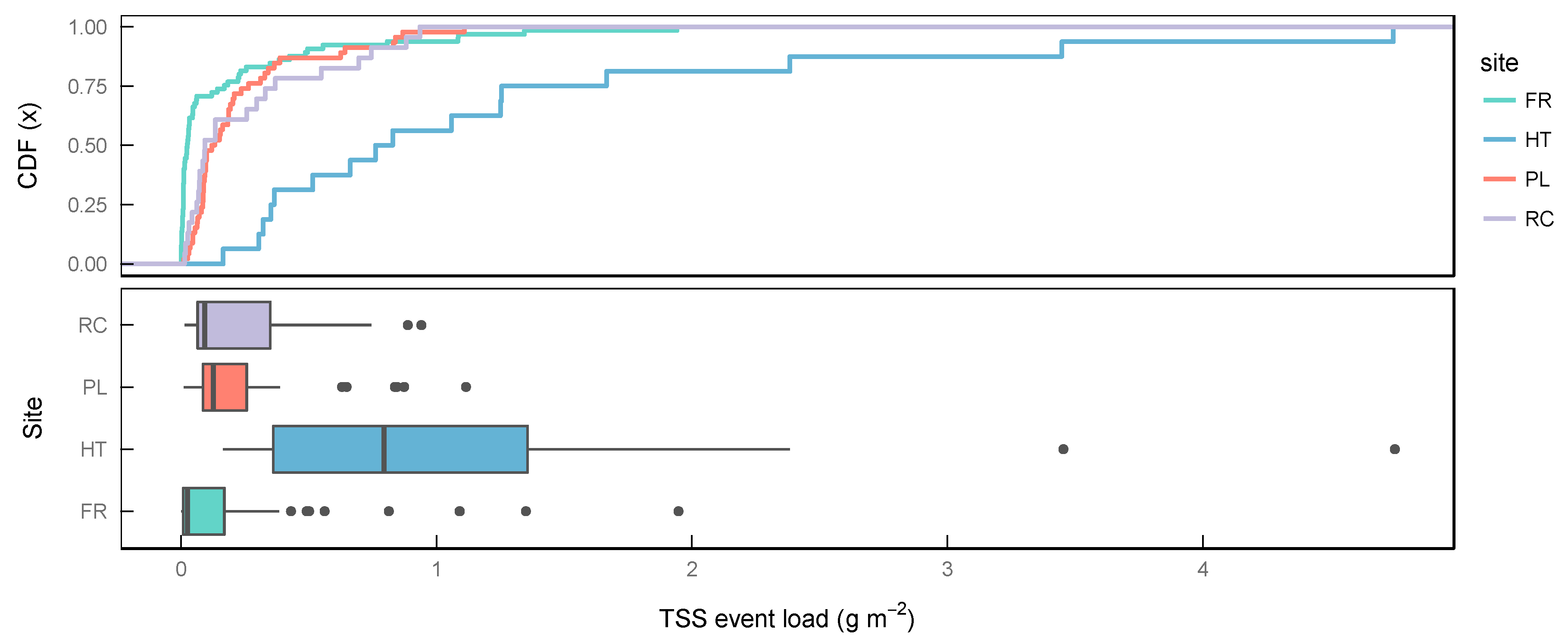
In this paper, the database of TSS event loads published in Reference [4] is used. In their work, the authors installed compact monitoring stations at the outlet of four common types of urban catchments and estimated TSS event loads by means of continuous turbidity sensors as a surrogate. The calculation of TSS event loads using turbidity data is shown in Reference [4]. Data from a flat roof (FR, 50 m², 65 events), a high traffic street (HT, 2.5 ha, 16 events), a parking lot (PL, 2350 m², 46 events) and a residential catchment (RC, 9.4 ha², 23 events) are available. A summary of descriptive statistics is given in

Table 1. Descriptive statistics (min, 0.1-, 0.25-, 0.5-, 0.75-, 0.9-percentiles, max, mean, standard deviation) of site-specific Total Suspended Solids (TSS) event loads (FR: Flat Roof, HT: High Traffic Street, PL: Parking Lot, RC: Residential Catchment).

Site	n		TSS Event Loads (g m−2)
		min	0.1-Perc	0.25-Perc	0.5-Perc	0.75-Perc	0.9-Perc	Max	Mean	sd
FR	65	0.001	0.002	0.008	0.024	0.169	0.492	1.942	0.174	0.358
HT	16	0.164	0.313	0.361	0.795	1.357	2.916	4.746	1.255	1.275
PL	46	0.011	0.046	0.086	0.126	0.257	0.633	1.109	0.230	0.255
RC	23	0.014	0.027	0.065	0.093	0.349	0.735	0.935	0.261	0.295

. Furthermore, Figure 1 depicts the distribution of site-specific TSS event loads as empirical cumulative distribution functions and box-plots, respectively.

2.2. Theoretical Distribution Functions

Site-specific distributions of empirical TSS event loads are derived and used to approximate theoretical distribution functions given in

Table 2. Theoretical distribution functions.

Name (Abbreviation)	Formula	Parameter
Exponential (exp)	$F\left(x\right)=\{\begin{array}{cc}\hfill 0,& \hfill x\le 0\\ \hfill 1-e^{-\alpha x},& \hfill x>0\end{array}$	α (rate)
Gamma (gamma)	$F\left(x\right)=\{\begin{array}{cc}\hfill 0,& \hfill x\le 0\\ \hfill \frac{b^p}{\mathsf{\Gamma }\left(p\right)}\times {{\displaystyle \int }}_0^x{t}^{p-1}{e}^{-bt}dt,& \hfill x>0\end{array}$	p (shape), b (rate)
Lognormal (lnorm)	$F\left(x\right)=\{\begin{array}{cc}\hfill 0,& \hfill x\le 0\\ \hfill \frac{1}{\sigma \sqrt{2\pi }}\times {{\displaystyle \int }}_0^x\frac{1}{t}{e}^{-\frac{1}{2}\left(\frac{\ln t-\mu }{\sigma }\right)}dt,& \hfill x>0\end{array}$	μ (meanlog), σ (sdlog)
Weibull (weibull)	$F\left(x\right)=\{\begin{array}{cc}\hfill 0,& \hfill x\le 0\\ \hfill 1-e^{-\alpha x^{\beta }},& \hfill x>0\end{array}$	α (scale), β (shape)

. For this purpose, distribution functions of type (i) Exponential; (ii) Gamma; (iii) Lognormal and (iv) Weibull are selected, as they closely correspond to observed distributions. In particular, these functions are only defined for positive values (x > 0) so that they inherently reflect one of the main characteristics of the empirical data. Additionally, parameters of the theoretical distribution functions are listed in the table. While the Exponential distribution has only one parameter, the Gamma, Lognormal and Weibull distributions offer two parameters to be estimated.

2.3. Distribution Fitting and Goodness-Of-Fit Assessment

To fit theoretical distribution functions to an empirical distribution, distribution parameters need to be optimized. In this study, parameters are estimated by maximum likelihood strategy (exact standard error model: μ = 0, σ = 1) because this also enables to analyze the standard error of estimated parameter. The likelihood function in general can be stated as follows (Equation (1)):

$$ℒ\left(\theta \right)=f(x_1,x_2,\dots ,x_n| \theta )={\displaystyle \prod }_{i=1}^{n}f(x_i|\theta )$$

(1)

with x_i the ith observation of variable X (i.e., TSS event loads), n is the total number of observations and f(|θ) the density function of the theoretical distribution function used. Parameters to be optimized are denoted by θ.

Since computation of likelihoods could result in very small numbers which may cause numerical precision problems, the logarithm of likelihoods (LL) is taken instead. Mathematically, loglikelihood values are a function of sample size and cannot alone indicate the goodness-of-fit. Therefore, once optimal parameters are estimated, the goodness-of-fit is evaluated by Kolmogorov-Smirnov (KS) and Anderson-Darling (AD) test statistics which are calculated according to

Table 3. Goodness-of-fit statistics used to evaluate the fitting (F_n denotes the empirical distribution function, F represents the fitted theoretical distribution function, sup abbreviates supremum which indicates the least element of x that is greater than or equal to all elements of x (“least upper bound”)).

Statistic (Abbreviation)	Formula
Kolmogorov-Smirnov (KS)	$D_n= \begin{array}{c}sup\\ x\end{array} \left|F_n\left(x\right)-F\left(x\right)\right|$	(2)
Anderson-Darling (AD)	$A^2=n {{\displaystyle \int }}_{-\infty }^{\infty }\frac{{\left(F_n\left(x\right)-F\left(x\right)\right)}^2}{F\left(x\right)\left(1-F\left(x\right)\right)}dF\left(x\right)$	(3)

. Fitting of theoretical distribution functions and numerical goodness-of-fit computations were done using R [29] and the package fitdistrplus [30].

In general, both tests are used to test whether a sample follows a specific distribution by calculating the maximum distance between empirical and theoretical distribution function. This means smaller test statistics indicate a lower numerical distance to the distribution analyzed. The AD test refines the KS test and gives more weight to the distribution tails. The tests are applied to decide whether the null hypothesis H₀ (“The sample follows a specified distribution”) can be accepted or must be rejected at a specified significance level. Alternatively, hypothesis H_A is defined as “the sample does not follow a specified distribution”. Critical values for the acceptance decision of the KS test are calculated according to Equation (4) for sample sizes > 35. For sample sizes below 35, critical values are obtained from Reference [31].

$$d_{\alpha }=\sqrt{\frac{-0.5 \ln \left(\frac{\alpha }{2}\right)}{\sqrt{n}}}, \mathrm{for} n>35$$

(4)

with sampling size n and significance level α.

2.4. Monte-Carlo Resampling Strategy to Determine Minimum Sample Size

A Monte-Carlo simulation based resampling strategy without replacement has been conducted to analyze the effect of different sample sizes on the quality of distribution fitting. Motivated by the idea to determine a minimum sample size required, the computational steps are as follows:

• Estimating parameters of lognormal distribution function by maximum likelihood taking all samples into account.
• Sampling k ($k\in \mathbb{N}, 0<k\le n$) events from all events n with 1000 repetitions. If less than 1000 repetitions are possible, all possible combinations are taken into account (Equation (3)).

  $$repetitions=MIN\left(\left(\begin{array}{c}n\\ k\end{array}\right), 1000\right)$$

  (5)

  with population n and sample size k.
• Computing of KS distance between empirical cumulative distribution function of sample and theoretical distribution function with estimated parameters for all repetitions.
• Computing of mean, standard deviations of KS distances for all repetitions.

The results are then interpreted and visually compared to the critical values for the Kolmogorov-Smirnov test statistic at 90% significance level. The minimum sample size is reached if addition of mean and the two standard deviations of KS distances from sampling are lower than the critical values.

3. Results

3.1. Distribution Fitting

Results of fitting theoretical distribution functions to the empirical TSS event load distribution are presented in

Table 4. Results of fitting empirical TSS load distribution functions to theoretical distribution functions (FR: Flat Roof, HT: High Traffic Street, PL: Parking Lot, RC: Residential Catchment, LL: LogLikelihood, AD: Anderson-Darling statistic A², KS: Kolmogorov-Smirnov statistic D_n; bold values indicate best-fit).

Site	Distr.	Goodness-Of-Fit			Parameter Estimates (Standard Error)
		LL	AD	KS	Rate	Shape	Meanlog	Sdlog	Scale
FR	exp	48.66	29.074	0.442 *	5.747 (0.713)	-	-	-	-
	gamma	88.29	2.254	0.186 *	1.994 (0.504)	0.347 (0.049)	-	-	-
	lnorm	89.9	0.806	0.099	-	-	−3.69 (0.301)	2.429 (0.213)	-
	weibull	92.05	1.123	0.131	-	0.484 (0.046)	-	-	0.077 (0.021)
HT	exp	−19.64	0.379	0.153	0.797 (0.199)	-	-	-	-
	gamma	−19.25	0.394	0.136	1.068 (0.412)	1.341 (0.428)	-	-	-
	lnorm	−18.18	0.192	0.128	-	-	−0.19 (0.228)	0.912 (0.161)	-
	weibull	−19.46	0.382	0.137	-	1.121 (0.208)	-	-	1.316 (0.312)
PL	exp	21.69	1.168	0.126	4.356 (0.642)	-	-	-	-
	gamma	22.03	1.279	0.157	5.093 (1.175)	1.169 (0.218)	-	-	-
	lnorm	25.31	0.398	0.116	-	-	−1.96 (0.146)	0.987 (0.103)	-
	weibull	21.72	1.203	0.137	-	1.030 (0.111)	-	-	0.233 (0.035)
RC	exp	7.91	1.011	0.222	3.833 (0.799)	-	-	-	-
	gamma	8.1	0.681	0.189	3.283 (1.120)	0.857 (0.219)	-	-	-
	lnorm	9.07	0.38	0.131	-	-	−2.03 (0.259)	1.243 (0.183)	-
	weibull	8.23	0.586	0.174	-	0.882 (0.142)	-	-	0.244 (0.061)

Note: * Rejecting H₀.

. It shows site- and distribution-specific goodness-of-fit values and estimated parameters.

All selected theoretical distribution functions were able to approximate the empirical distribution with statistical significance except for the Exponential and the Gamma distribution at site FR (H₀ gets rejected). These two functions are not able to sufficiently reflect the initially steep gradient and subsequent moderate gradient of the empirical distribution (cf. Figure 1).

Using the Weibull distribution which basically extends the Exponential distribution function with an additional parameter, clearly improves the fitting. The application of Weibull and Gamma distribution lead to comparable results which is indicated by similar goodness-of-fit measures. Highest goodness-of-fit at site HT, PL and RC is obtained with the Lognormal distribution that accordingly approximates the underlying dataset best. According to the loglikelihood, the Weibull distribution is best suited to describe the empirical distribution at site FR. However, the difference to Lognormal is marginal.

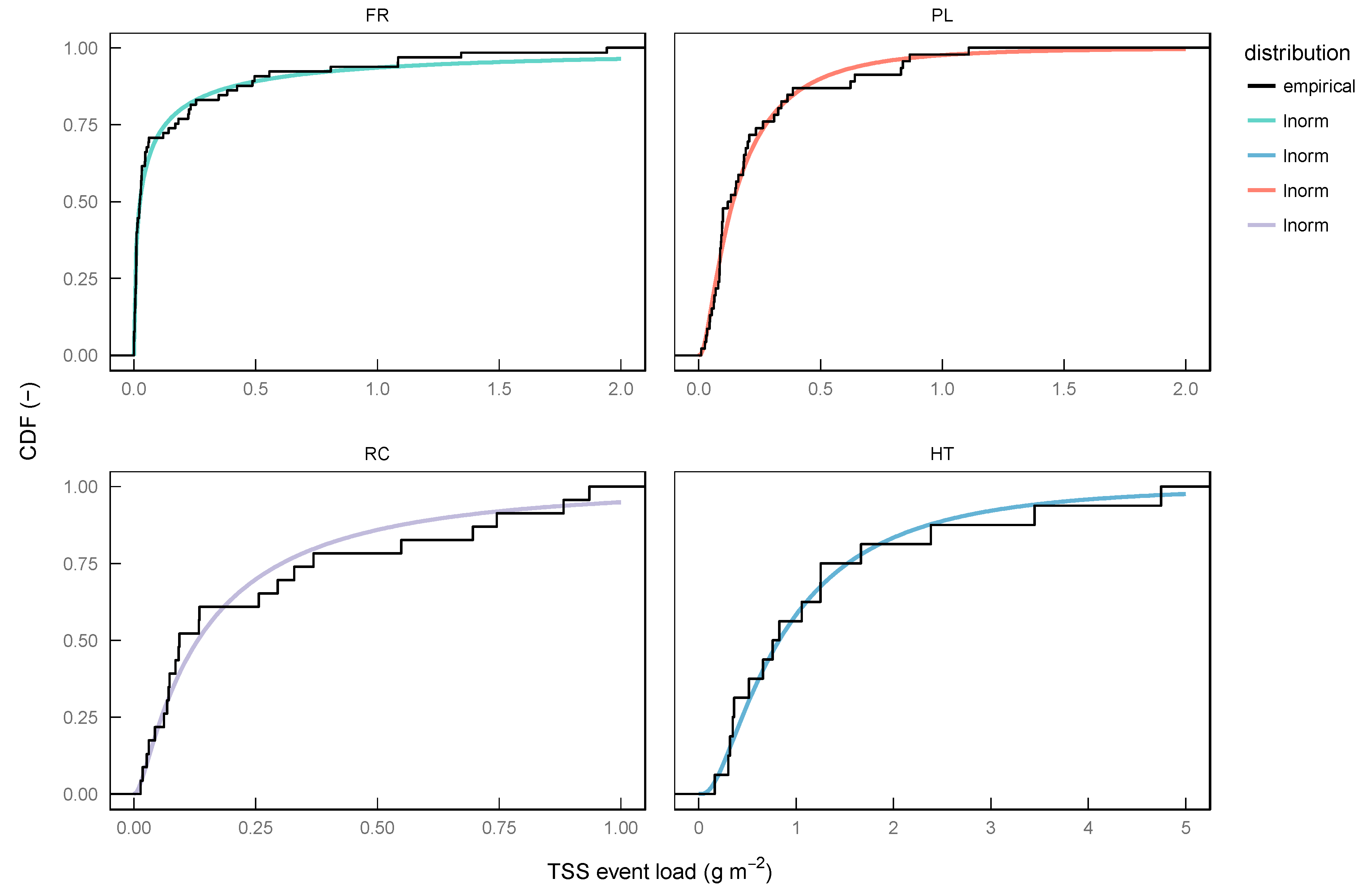
The goodness-of-fit of the Lognormal distribution varies between sites. Figure 2 illustrates the approximation with Lognormal distribution function for all sites. Sites FR and PL show the best visual fitting. Goodness-of-fit at sites RC and HT is poorer, which however is also influenced by sharp steps of the empirical distribution functions due to low sample size.

Comparing the fitted parameters also indicates that distributions of site PL and RC are comparable which is also visually confirmed by their empirical distribution functions (cf. Figure 1).

Table 5. Results of fitting empirical TSS load distribution functions grouped by year to lognormal distribution function (FR: Flat Roof, PL: Parking Lot, LL: LogLikelihood, AD: Anderson-Darling statistic A², KS: Kolmogorov-Smirnov statistic D_n).

Site	Year	n	Distr.	Goodness-Of-Fit			Parameter Estimates (Standard Error)
				LL	AD	KS	Meanlog	Sdlog
FR	all years	65	lnorm	89.9	0.806	0.099	−3.69 (0.301)	2.429 (0.213)
	2015	25	lnorm	24.54	0.64	0.138	−2.99 (0.359)	1.80 (0.254)
	2014	17	lnorm	41.63	0.288	0.142	−5.04 (0.786)	3.24 (0.556)
	2013	23	lnorm	32.52	0.365	0.12	−3.45 (0.388)	1.86 (0.274)
PL	all years	46	lnorm	25.31	0.398	0.116	−1.96 (0.146)	0.987 (0.103)
	2014	30	lnorm	23.76	0.616	0.167	−2.08 (0.161)	0.88 (0.114)
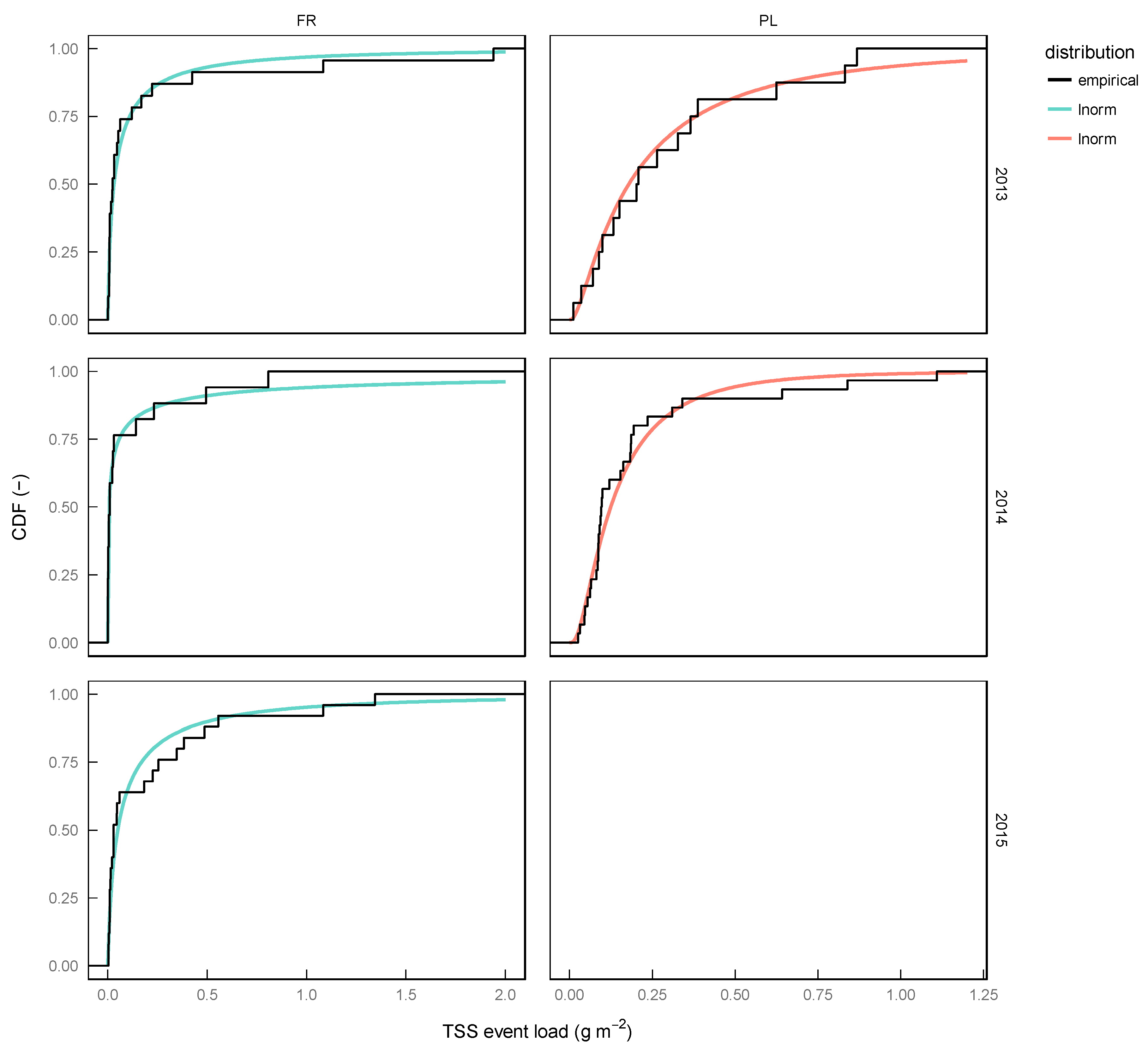
	2013	16	lnorm	2.93	0.243	0.105	−1.72 (0.281)	1.12 (0.199)

shows results of fitting the Lognormal distribution to TSS event load distributions grouped by year. Sites FR and PL are considered only as they provide sufficient samples per group. The goodness-of-fit is given for each individual group and compared to the original sample from all years. Additionally, the goodness-of-fit is shown in Figure 3.

The results show that also subsamples can be well approximated by Lognormal distribution. According to the KS statistic, for both sites the year 2013 has been fitted best. Only the AD statistic of the year 2014 for site FR indicates a slightly better fit which is caused by a relative low maximum load in this year (2013: 1.94 gm⁻², 2014: 0.8 gm⁻², 2015: 1.34 gm⁻²). The optimized parameters of the Lognormal distribution for both sites highlight the individuality of each year as they strongly vary. This is also confirmed by the spread of goodness-of-fit values.

3.2. Minimum Sample Size

The results obtained from the Monte-Carlo-based sampling are shown in Figure 4. It shows the mean (colored solid line) and regions of one and two standard deviations (grey shaded areas) of Kolmogorov-Smirnov’s statistic as function of sample size for site FR and PL. Furthermore, critical values for the 90% significance level are illustrated (black solid line).

It can be seen that the mean of the calculated goodness-of-fit values improves with increasing sample size and approximates to the value obtained when all samples are taken into account (FR: 0.099, PL: 0.12). The standard deviation decreases with increasing sampling size by implication. With respect to critical values for 90% confidence level, accepting the null hypothesis H₀ (“The data follow the Lognormal distribution”) generally requires Kolmogorov-Smirnov’s D_n to be approximately below the μ + 2σ threshold, which is satisfied for minimum sample sizes of about 40 at site FR and of roughly 30 at site PL. It can be legitimately assumed that simulated KS statistics follow a normal distribution which according to the empirical rule (The empirical rule states that for a normal distribution 99.7% of the data fall within three standard deviations, 95% are within two standard deviations and 68% fall within one standard deviation [31]) consequently implies that more than approximately 95% of samples lead to KS statistics lower than 0.188 at site FR and 0.211 at site PL. Narrowing the uncertainty range to the upper limit of μ + σ threshold results in KS statistics of 0.159 at site FR and 0.176 at site PL (approx. more than 68% of samples are within this range).

4. Discussion

4.1. Distribution Fitting

The results of the distribution fitting suggest, that theoretical distributions are general applicable to replicate empirical TSS event loads from small urban sites. Among the functions analyzed, the Exponential function has the least flexibility because it only provides one parameter to be fitted. This explains the poor approximation results. A statistical significant description of TSS event load distributions therefore requires at least a two-parameter distribution. The Lognormal distribution has shown to be best suited for sites investigated in this study. However, the goodness-of-fit has been found to be site-specific. On the one hand, this might be caused by site-specific varying sample sizes, which lead to more pronounced steps in the empirical distribution function. On the other hand, this also could reflect a site-specific behavior, which is expressed by the shape of distribution function. For example, the monitored small roof catchment has significantly more events with low loads. This characteristic is less pronounced for the other catchments. Consequently, this highlights the sensitivity of sampling characteristics which is induced by the utilized database and corresponding study sites. In the present study the database available does not cover all events of an entire year mainly due to measurement issues and predefined rainfall-runoff criteria for event selection [4]. However, rainfall-runoff events are affected by numerous environmental variables and generally occur randomly in time, space and intensity. Therefore, although the event database grouped by year undoubtedly is incomplete, the approach reflects natural variability in which the number of events per year and their characteristics change. As a consequence, fitting of a theoretical distribution function should therefore prioritize sample size over sampling period (cf. Section 4.2). Sample sizes for HT (n = 16) and RC (n = 23) are assumed to be insufficient to robustly fit a theoretical distribution.

Since TSS event loads from small sites follow a Lognormal distribution, this should be taken into account by stormwater quality modelling approaches. The results show that catchment size and land usage affect the parameterization of distribution function. However, the transferability of parameterized distribution functions could not be verified yet due to lack of data. Comparing the parameterized lognormal distributions with data from similar catchments would be of high relevance and would greatly contribute to further analysis of the stochasticity of stormwater quality.

4.2. Minimum Sample Size

Generally, the dataset confirms that the more samples are taken into account, the more precise the estimates get which as a matter of fact is the basic assumption for any statistical significance test. In order to determine the sample size which leads to accepting the null hypothesis H₀ with high probability, it is suggested to choose at least the minimum of 40 samples because of (i) the chance of having a sample which can be statistically represented by the Lognormal distribution is high (>95%) and (ii) the mean of KS statistic in this case only slightly differs from the optimal value taking all samples into account (0.131 > 0.099 at site FR and 0.122 > 0.12 at site PL). However, the choice of criteria remains subjective and might be adapted as further data becomes available.

Of course, using more data to approximate the Lognormal distribution may probably lead to more appropriate fitting results, but this requires to provide more samples which in turn needs more measurement data. The criteria proposed therefore represent a compromise solution between measurement duration and quality of approximation.

5. Conclusions

Empirical TSS event load distributions of four small common types of urban catchments (Flat Roof (FR), Parking Lot (PL), Residential Catchment (RC), High Traffic Street (RC)) are successfully described by theoretical distribution functions. The goodness-of-fit was evaluated and effects of sampling sizes were investigated. From the analysis, it was found that:

• The Lognormal distribution function is most expressive to approximate empirical TSS event load distributions at all experimental sites.
• Successfully derived and fitted distribution functions provide a closed characterization of TSS event load distributions allowing to intra- and extrapolate of probabilistic event characteristics not observed.
• A robust fitting should prioritize sample size over sampling period.
• Roughly 40 events are required to reasonably fit the Lognormal distribution. Using more samples potentially improves the goodness-of-fit but subsequently requires to extend the duration of cost-intensive monitoring campaigns.

When applying the concept of probabilistic description of TSS event loads based on theoretical distribution function, the results of this study may also support the evaluation of stormwater quality runoff monitoring campaigns with respect to their duration-to-information ratio. Data from an ongoing monitoring campaign may be used to update the parameters of the theoretical distribution function which in turn can be analyzed in terms of their relative change. If changes are not significant, the duration of monitoring might be shortened. However, the minimum sample size should be taken into account. In addition, the fitted distribution functions provide an excellent basis to calibrate urban stormwater quality models by focusing on probabilistic TSS event load characteristics. This in turn improves a more realistic pollutant load estimation and enhances stormwater emission control.

References

- Allen Burton, G.; Pitt, R. Stormwater Effects Handbook: A Toolbox for Watershed Managers, Scientists, and Engineers; CRC Press: Boca Raton, FL, USA, 2001; ISBN 978-0-87371-924-7. [Google Scholar]
- Zoppou, C. Review of urban storm water models. Environ. Model. Softw. 2001, 16, 195–231. [Google Scholar] [CrossRef]
- Niazi, M.; Nietch, C.; Maghrebi, M.; Jackson, N.; Bennett, B.R.; Tryby, M.; Massoudieh, A. Storm Water Management Model: Performance Review and Gap Analysis. J. Sustain. Water Built Environ. 2017, 3, 04017002. [Google Scholar] [CrossRef]
- Leutnant, D.; Muschalla, D.; Uhl, M. Stormwater Pollutant Process Analysis with Long-Term Online Monitoring Data at Micro-Scale Sites. Water 2016, 8, 299. [Google Scholar] [CrossRef]
- Gruber, G.; Winkler, S.; Pressl, A. Quantification of pollution loads from CSOs into surface water bodies by means of online techniques. Water Sci. Technol. 2004, 50, 73–80. [Google Scholar] [CrossRef] [PubMed]
- Bertrand-Krajewski, J.-L. TSS concentration in sewers estimated from turbidity measurements by means of linear regression accounting for uncertainties in both variables. Water Sci. Technol. 2004, 50, 81–88. [Google Scholar] [CrossRef] [PubMed]
- Caradot, N.; Sonnenberg, H.; Rouault, P.; Gruber, G.; Hofer, T.; Torres, A.; Pesci, M.; Bertrand-Krajewski, J.-L. Influence of local calibration on the quality of online wet weather discharge monitoring: Feedback from five international case studies. Water Sci. Technol. 2015, 71, 45. [Google Scholar] [CrossRef] [PubMed]
- Métadier, M.; Bertrand-Krajewski, J.-L. The use of long-term on-line turbidity measurements for the calculation of urban stormwater pollutant concentrations, loads, pollutographs and intra-event fluxes. Water Res. 2012, 46, 6836–6856. [Google Scholar] [CrossRef] [PubMed]
- Bertrand-Krajewski, J.L.; Chebbo, G.; Saget, A. Distribution of pollutant mass vs volume in stormwater discharges and the first flush phenomenon. Water Res. 1998, 32, 2341–2356. [Google Scholar] [CrossRef]
- Di Modugno, M.; Gioia, A.; Gorgoglione, A.; Iacobellis, V.; la Forgia, G.; Piccinni, A.; Ranieri, E. Build-Up/Wash-Off Monitoring and Assessment for Sustainable Management of First Flush in an Urban Area. Sustainability 2015, 7, 5050–5070. [Google Scholar] [CrossRef] [Green Version]
- Bertrand-Krajewski, J.-L. Stormwater pollutant loads modelling: Epistemological aspects and case studies on the influence of field data sets on calibration and verification. Water Sci. Technol. 2007, 55, 1–17. [Google Scholar] [CrossRef] [PubMed]
- Egodawatta, P.; Thomas, E.; Goonetilleke, A. Understanding the physical processes of pollutant build-up and wash-off on roof surfaces. Sci. Total Environ. 2009, 407, 1834–1841. [Google Scholar] [CrossRef] [PubMed] [Green Version]
- Al Ali, S.; Bonhomme, C.; Dubois, P.; Chebbo, G. Investigation of the wash-off process using an innovative portable rainfall simulator allowing continuous monitoring of flow and turbidity at the urban surface outlet. Sci. Total Environ. 2017, 609, 17–26. [Google Scholar] [CrossRef] [PubMed]
- Alias, N.; Liu, A.; Goonetilleke, A.; Egodawatta, P. Time as the critical factor in the investigation of the relationship between pollutant wash-off and rainfall characteristics. Ecol. Eng. 2014, 64, 301–305. [Google Scholar] [CrossRef] [Green Version]
- Egodawatta, P.; Thomas, E.; Goonetilleke, A. Mathematical interpretation of pollutant wash-off from urban road surfaces using simulated rainfall. Water Res. 2007, 41, 3025–3031. [Google Scholar] [CrossRef] [PubMed] [Green Version]
- Muthusamy, M.; Tait, S.; Schellart, A.; Beg, M.N.A.; Carvalho, R.F.; de Lima, J.L.M.P. Improving understanding of the underlying physical process of sediment wash-off from urban road surfaces. J. Hydrol. 2018, 557, 426–433. [Google Scholar] [CrossRef] [Green Version]
- Zhao, H.; Jiang, Q.; Xie, W.; Li, X.; Yin, C. Role of urban surface roughness in road-deposited sediment build-up and wash-off. J. Hydrol. 2018, 560, 75–85. [Google Scholar] [CrossRef]
- Liu, A.; Egodawatta, P.; Guan, Y.; Goonetilleke, A. Influence of rainfall and catchment characteristics on urban stormwater quality. Sci. Total Environ. 2013, 444, 255–262. [Google Scholar] [CrossRef] [PubMed] [Green Version]
- Shaw, S.B.; Walter, M.T.; Steenhuis, T.S. A physical model of particulate wash-off from rough impervious surfaces. J. Hydrol. 2006, 327, 618–626. [Google Scholar] [CrossRef]
- Hong, Y.; Bonhomme, C.; Le, M.-H.; Chebbo, G. A new approach of monitoring and physically-based modelling to investigate urban wash-off process on a road catchment near Paris. Water Res. 2016, 102, 96–108. [Google Scholar] [CrossRef] [PubMed]
- Le, M.-H.; Cordier, S.; Lucas, C.; Cerdan, O. A faster numerical scheme for a coupled system modeling soil erosion and sediment transport. Water Resour. Res. 2015, 51, 987–1005. [Google Scholar] [CrossRef] [Green Version]
- Delestre, O.; Darboux, F.; James, F.; Lucas, C.; Laguerre, C.; Cordier, S. FullSWOF: Full Shallow-Water equations for Overland Flow. J. Open Source Softw. 2017, 2, 448. [Google Scholar] [CrossRef] [Green Version]
- Shaw, S.B.; Stedinger, J.R.; Walter, M.T. Evaluating urban pollutant buildup/wash-off models using a Madison, Wisconsin catchment. J. Enviorn. Eng. 2009, 136. [Google Scholar] [CrossRef]
- Gunawardena, J.M.A.; Liu, A.; Egodawatta, P.; Ayoko, G.A.; Goonetilleke, A. Influence of Traffic and Land Use on Urban. Stormwater Quality—Implications for Urban Stormwater Treatment Design; SpringerBriefs in Water Science and Technology; Springer: Singapore, 2018; ISBN 978-981-10-5301-6. [Google Scholar]
- Van Buren, M.A.; Watt, W.E.; Marsalek, J. Application of the log-normal and normal distributions to stormwater quality parameters. Water Res. 1997, 31, 95–104. [Google Scholar] [CrossRef]
- Haan, C.T. Statistical Methods in Hydrology, 1st ed.; Iowa State University Press: Ames, IA, USA, 1977; ISBN 978-0-8138-1510-7. [Google Scholar]
- eWater MUSIC Version 6 Documentation and Help Home. Available online: https://wiki.ewater.org.au/display/MD6 (accessed on 15 May 2018).
- Toranjian, A.; Marofi, S. Evaluation of statistical distributions to analyze the pollution of Cd and Pb in urban runoff. Water Sci. Technol. 2017, 75, 2072–2082. [Google Scholar] [CrossRef] [PubMed]
- R Core Team. R: A Language and Environment for Statistical Computing; R Foundation for Statistical Computing: Vienna, Austria, 2018. [Google Scholar]
- Delignette-Muller, M.L.; Dutang, C. Fitdistrplus: An R package for fitting distributions. J. Stat. Softw. 2015, 64, 1–34. [Google Scholar] [CrossRef]
- Hedderich, J.; Sachs, L. Angewandte Statistik: Methodensammlung Mit R; 14. überarb. und erg. Aufl.; Springer: Heidelberg, Germany, 2012; ISBN 978-3-642-24400-1. [Google Scholar]
Figure 1.
Empirical cumulative distribution functions and boxplots of site-specific monitored Total Suspended Solids (TSS) event loads (FR: Flat Roof, HT: High Traffic Street, PL: Parking Lot, RC: Residential Catchment).
Figure 2.
Approximation of empirical TSS event load distribution function with lognormal distribution function at all sites.
Figure 3.
Approximation of empirical TSS event load distribution function grouped by year with lognormal distribution function at sites FR and PL.
Figure 4.
Mean and regions of one and two standard deviations of Kolmogorov-Smirnov’s statistic as function of sample size from Monte-Carlo-based sampling for sites Flat Roof (FR) and Parking Lot (PL). Critical values for 90% confidence are indicated as black solid line.