Application of Terrestrial Laser Scanning to Tree Trunk Bark Structure Characteristics Evaluation and Analysis of Their Effect on the Flow Resistance Coefficient

Abstract

The paper presents an original method for the evaluation of bark structure characteristics of tree trunks on the basis of terrestrial laser scanning data. Measurements testing the method proposed were performed in laboratory conditions for trunks of pine (Pinus sylvestris L.) and oak (Quercus robur L.). The laser scanner used was a FARO Focus 3D. The scanning was carried out in two variants for natural trunks (variant I: samples Oak-I, Pine-I) and for trunks wrapped in foil (variant II: samples Oak-II, Pine-II). The point clouds obtained were combined into a three-dimensional (3D) model, filtered, and exported to the *.xyz format in SCENE (v. 5×) software provided by FARO. For calculation of the bark structure characteristics the geoprocessing Tree Trunk Bark Structure Model (TTBSM) operating in the ArcGIS environment was developed. The mean bark height factor (BHF) of the natural pine and oak tree trunks was calculated to be 0.39 cm and 0.37 cm, while the values for the trunks wrapped in foil were 0.27 cm and 0.25 cm, respectively. The BHF of the tree trunks wrapped in foil varied in the range 0.26–0.28 cm and 0.24–0.26 cm for pine and oak, respectively, while for the natural tree trunks the range was 0.38–0.46 cm and 0.35–0.38 cm for pine and oak, respectively. The effect of BHF on the flow resistance was evaluated in a measuring trough and proved to be significant. The coefficient of flow resistance was on average 20% higher for the natural tree trunks than for those foil-wrapped.

1. Introduction

Many authors have carried out research on the impact of vegetation on flow conditions in open channel flow. The studies concern derivation of theoretical principles of the mathematical modeling of the phenomenon [1,2,3,4,5], numerical modeling with models of varying complexity [6,7,8], flume experiments to verify models of vegetation roughness [9,10,11], and in situ floodplain roughness estimations [12]. Remote sensing methods were used to acquire data used in hydraulic modeling [13].

The roughness calibration of floodplains and channels is an important issue in flood studies [14]. Riparian vegetation plays a crucial role affecting the floodplain hydraulic roughness [15]. Vegetation roughness, and more specifically forest roughness, is a necessary component in more accurate determination of flood dynamics [16]. Tree trunks are major contributors to the roughness coefficient in a densely wooded floodplain. Petryk and Bosmajian [17] have developed a method for determination of the roughness coefficient on the basis of the vegetation density. Trees density can be determined by measuring the number of trees and trunk sizes in a representative-sample area [18]. From the hydrological point of view, measurement of canopy structure must be nondestructive and applicable over a broad area to allow investigation of seasonal fluctuations [19].

The floodplain drag coefficient sums up pressure and friction drag. The pressure, or form drag, is caused by the difference between the high pressure upstream and low pressure downstream of an element [20]. For open-channel flow the friction factor $f_p$ for riparian vegetation is defined as:

$$f_p=\frac{4·h·d_p}{a_x·a_y}·C_d$$

(1)

where $h$ is the flow depth (m), $d_p$ is the diameter of the plant (m), $a_x$ is the longitudinal distance between the plants (m), $a_y$ is the lateral distance between the plants (m), and $C_d$ is the plants’ drag coefficient.

The drag coefficient $C_d$ depends on the separation characteristics of the cylinder boundary layer and is a function of the cylinder Reynolds number:

$$Re=\frac{u·d_p}{v}$$

(2)

where $u$ denotes mean velocity and $v$ denotes the fluid kinematic viscosity (e.g., [21]).

This type of formulation was originally derived for rigid cylinders simulating tall trees, but its use has been extended to other types of vegetation. However, for natural plants the determination of projected area and drag coefficient is difficult. The hydraulic characteristics $d_p$, $a_x$, and $a_y$ are determined on the basis of field measurements in the area of the water flow. Floodplains and riparian zones of rivers and streams are usually covered by groups of trees or bushes.

Estimation of the flow resistance of trees $F_d$ is complex due to the variability in tree morphology [22]. In fluid mechanics, the drag force, which acts on a surface area $A_d$ measured perpendicular to the direction of the flow, may be defined as:

$$F_d=\frac{1}{2}·\rho ·C_d·A_d·u^2$$

(3)

where $\rho$ is the density of the fluid [kg·m⁻³], $A_d$ is the vegetal area ($A_d=h·d_p$) (m²).

The main basis for hydraulic calculations of the river flow, where the structure of high vegetation is taken into account, is that water flow resistance is the same as vegetation resistance, which occur when water overflows regularly distributed vegetation with averaged geometric parameters and averaged effect of roughness of plants on the coefficient $C_d$. It is important to correctly determine these parameters.

At present to describe the canopy structure of flood valleys satellite multispectral data [15] and airborne (ALS) [23,24,25] and terrestrial laser scanning data (TLS) are used [26]. Laser scanning is an active remote-sensing technique, which provides high-resolution spatial data [27]. ALS data were used to explore the tree morphometric properties from riparian zones such as tree position, tree height, trunk location, and tree spacing [28]. Methods based on ALS data do not allow detailed analysis of tree trunk and branch parameters. Nowadays TLS technique is widely used in forestry applications [29,30]. TLS can produce high-resolution three-dimensional point clouds over scales of meters to kilometers with centimeter or sub-centimeter precision on geometric parameters of trees [31,32]. Methods based on TLS data have been used for automatic measurement of forest inventory attributes [27,33]. Numerous studies can be found in literature on calculation of the diameter at breast height (DBH), the height of the tree, the volume of wood, stem ovality, structure, and damage of the bark, tree topology, branch angles, and diameters [34,35]. Othmani et al. [30,36], Brolly and Király [27], and Lin and Herold [37] have confirmed the possibility of identification of tree species using TLS data on the basis of 3D bark texture analysis. It has been proven that TLS is capable of fulfilling such tasks as: retrieval of leaf area density [38], derivation of vertical crown profile [39], and estimation of above-ground biomass [40]. Sioma et al. [41] were used 3D vision system to characterizing spatial patterning of bark texture.

TLS is used for the purpose of extracting canopy parameters relevant for parameterization of the flow resistance equations [26]. Laser scanning is an efficient technique to obtain data on the scale of a single tree [27,28]. Beside TLS, a commonly used method is Structure from Motion, which can be used to make 3D models from photographs [42] or video frames [43]. Considering the variety of tree trunk surfaces, it is very important to determine the drag characteristics of real tree trunks with various barks to a high accuracy. Estimation of the drag coefficient of a real tree considering the vertical stand structure of the trunk, branches, and leaves has been studied by Tanaka et al. [44]. According to these authors, reliable determination of the vegetation flow resistance requires the millimeter scale resolution that can be provided by terrestrial laser scanning [45,46]. Roughness of the tree trunk surface is known to affect their flow resistance; however, hitherto its effect has been neglected and $C_d$ values the same as for smooth cylinders have been applied. The progress in remote sensing technology has provided an opportunity for detailed studies taking into account the tree bark structure.

The aims of the study were: (i) to develop a model (Tree Trunk Bark Structure Model–TTBSM) for supporting the calculations of tree trunk bark characteristics on the basis of the data from terrestrial laser scanning in the ArcGIS 10.5 (ESRI Inc., Redlands, CA, USA) environment; (ii) to analyze the effect of bark structure on the drag force in a forested zone.

2. Materials and Methods

2.1. Characterization of the Tree Trunks Used

The effect of bark structure of tree trunks on the flow resistance coefficient was evaluated for the trunks of Scots pine (Pinus sylvestris L.) and common oak (Quercus robur L.). Scots pine is the most common tree species in Polish forests, representing over 58.2% of trees in forested areas. Pines often grow on sandy soil in alluvial river valleys. The second most frequent tree species in Polish forests is common oak, with a frequency of 7.7%. Because of its ecological demands this species grows in wet and marshy habitats. The measurements were performed for freshly cut bottom fragments of tree trunks of about 0.2 m in diameter and 0.5 m in height. The tree trunk samples were weighed and their diameters and circumferences were measured (

Table 1. Basic parameters of tree trunk samples used for measurements.

Parameters		Units	Tree Species
			Pine	Oak
Height		(m)	0.5	0.5
Weight		(kg)	9.3	11.2
Circumference
	bottom	(m)	0.60	0.67
	mid	(m)	0.62	0.68
	top	(m)	0.56	0.64
Diameter
	bottom	(m)	0.190	0.205
	top	(m)	0.185	0.210

).

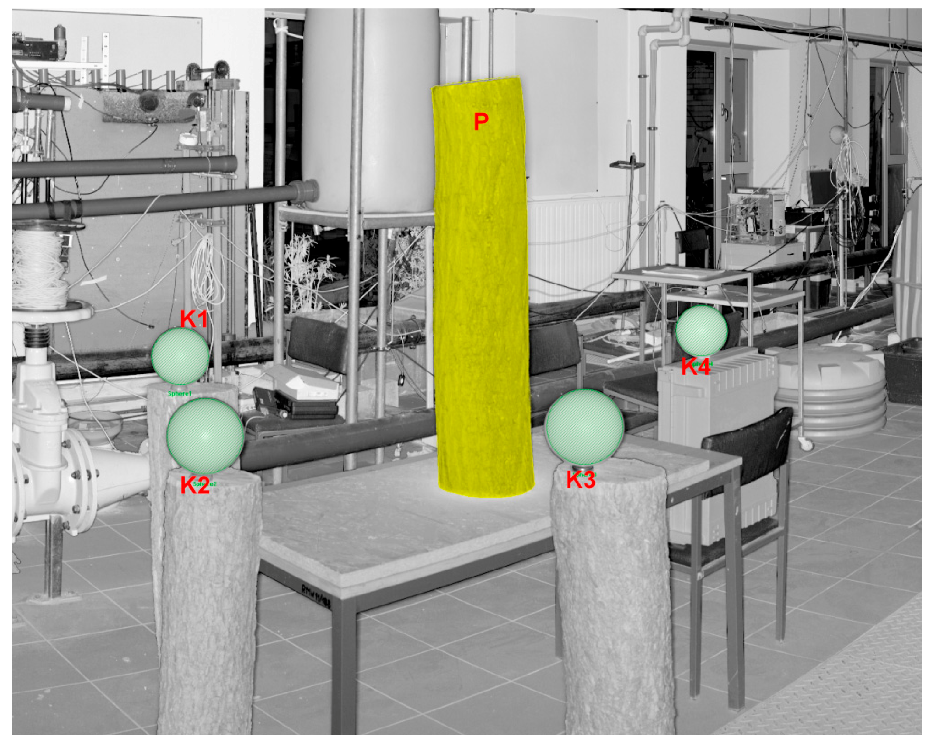
2.2. Tree Trunk Scanning

The surfaces of the tree trunks were subjected to scanning. To ensure their stability in the process they were attached to a special board and set on a table (Figure 1). Around the tree trunk to be scanned four white reference balls were placed (K1–K4) that permitted later combination of the scans into a single 3D model. Each fragment of the tree trunk was scanned from three sites localized in such a way that a 3D model of the trunk could be obtained. The scanner was positioned at a distance of 2.2–2.5 m from the trunk. The positions of the reference balls with respect to one another and to the trunk were unchanged.

In order to evaluate the effect of tree trunk bark structure on the flow resistance, the scanning was performed in two variants. At first the tree trunks were wrapped up with a stretch foil and scanned. The applied foil was made of stretchable polyethylene of low density (LLDPE). The foil had a thickness of 23 μm and stretch of 150%. Due to its elasticity and stretching during wrapping, the foil adhered very tightly to the trunk thus eliminating microrelief of the trunk bark. Foil wrapped trunks simulated smooth trunks without bark. In the second variant of the experiment the tree trunks in their natural form—without foil—were scanned. This sequence of measurements was chosen on purpose to minimize disturbances to the trunks’ positions as the procedures of wrapping carry greater risk of disturbance than the unwrapping. The scanner used was FARO Focus 3D (Lake Mary, FL, USA); its parameters are given in

Table 2. Scanner specification

Ranging Unit
Range	0.6–120 m
Measurement speed	122,000–976,000 points s−1
Ranging error	±2 mm at 10 m
Laser (Optical Transmitter)
Laser power (cw Ø)	20 mW
Wavelength	905 nm
Beam divergence	0.19 mrad (0.011°)
Beam diameter at exit	3.0 mm, circular
Deflection Unit
Vertical field of view	305°
Horizontal field of view	360°
Vertical step size	0.009° (40,960 3D pixel on 360°)
Horizontal step size	0.009° (40,960 3D pixel on 360°)
Max. vertical scan speed	5820 rpm or 97 Hz

.

The scanner settings were: resolving power ¼, quality 4×, rate 122 thousand points s⁻¹, vertical range 10–25 degrees, horizontal range 0–60 degrees. The used scanner settings allowed point clouds with spatial resolution of 50 points/cm² to be obtained.

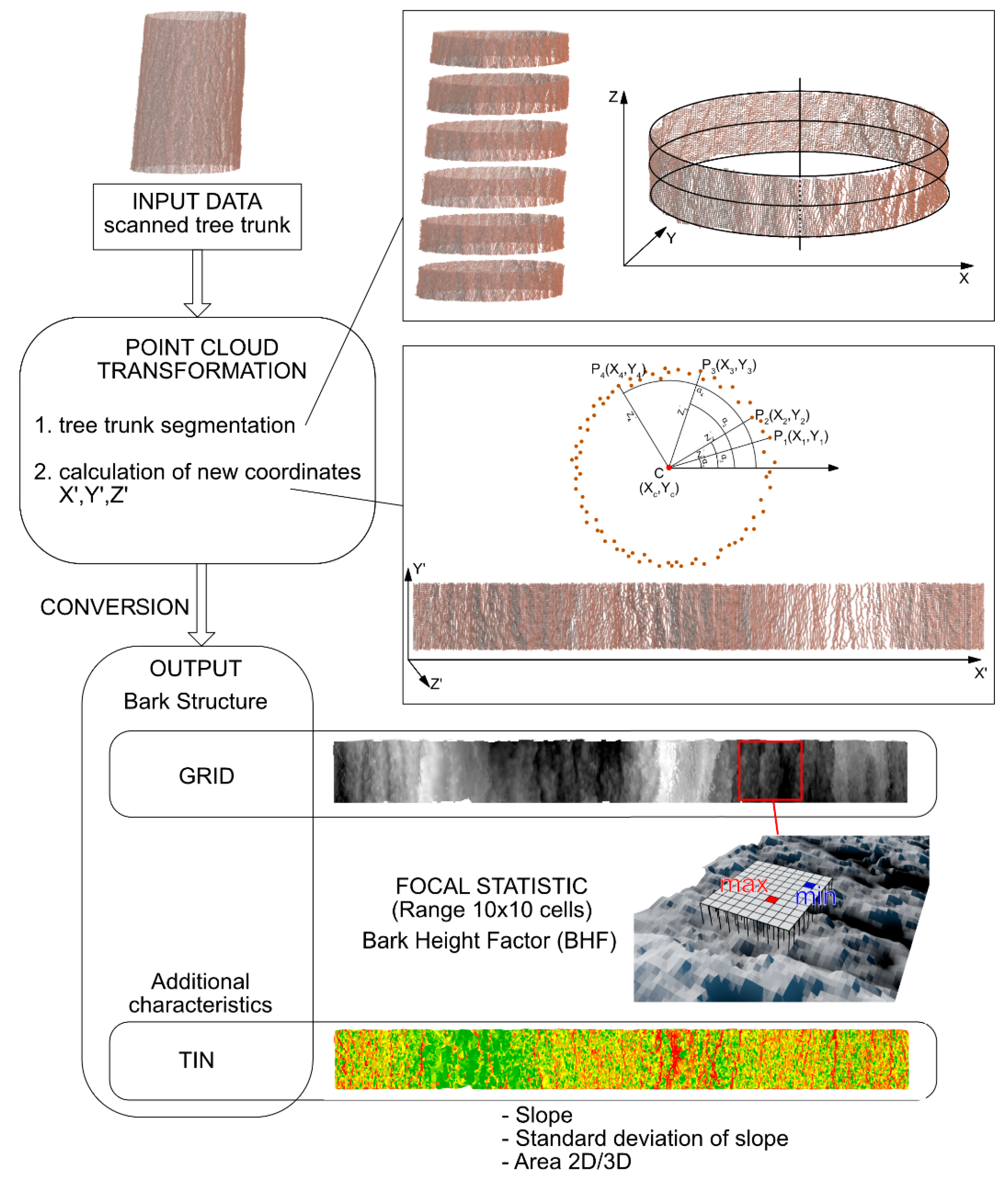
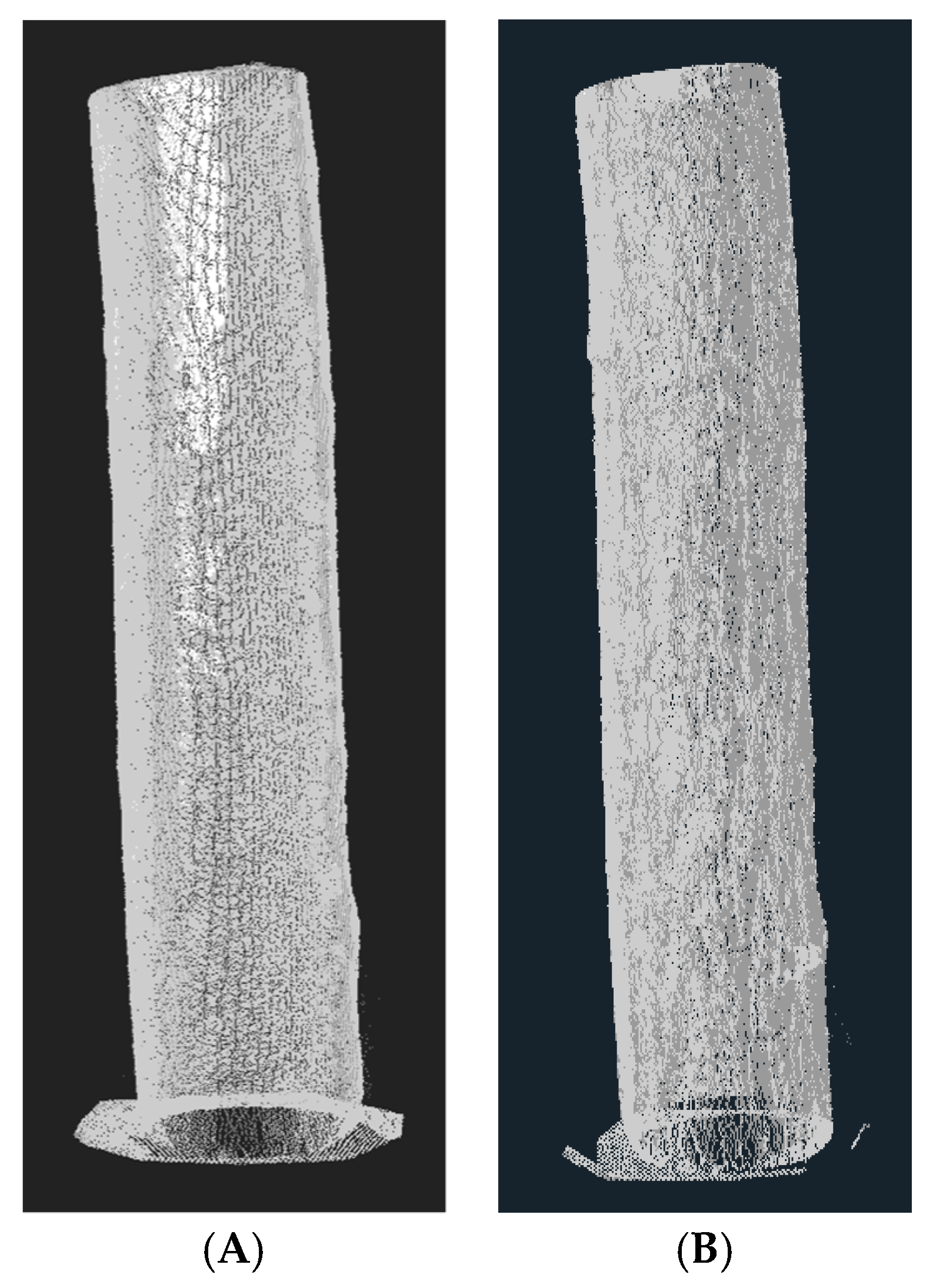
2.3. Data Preprocessing

The point clouds obtained from individual scans were combined in a single 3D model using the SCENE (v. 5.0) software from FARO. The SCENE software was necessary for reading in the scan files, for detection of reference balls and combination of the scans in one 3D model. Then the models were subjected to preliminary filtration and the scanning area was reduced to the trunk. Finally the point clouds obtained were exported to a file of *.xyz format, containing information on the 3D coordinates of each point and on the intensity of reflection recorded as grades of grey.

2.4. Data Processing—Calculation of Tree Trunk Bark Characteristics

In order to calculate bark characteristics of the tree trunks GIS tools were used. The idea was to use similar techniques as in physiography studies to describe terrain roughness with Digital Terrain Models but on the micro scale. In order to achieve this, the input data, in the form of point clouds of scanned tree trunks, should be unwrapped to a 2.5D surface. The TTBSM was created to make this time-consuming process fully automated. The scheme of the model processing is shown in Figure 2.

The first step was to import the scanned tree trunk point cloud data in .XYZ format. The next step was to unwrap the point cloud into a 2.5D form. The transformations of point clouds making 3D models of tree trunks (X, Y, Z) to the calculation form (X′, Y′, Z′) were performed according to Formulas (4)–(6).

$$X_i^{\prime }=\frac{2\pi ·{\alpha }_i·\overline{Z_i^{\prime }}}{360}$$

(4)

$$Y_i^{\prime }=Z_i$$

(5)

$${\mathrm{Z}}_i^{\prime }=\sqrt{{\left(X_i-X_C\right)}^2+{\left(Y_i-Y_C\right)}^2}$$

(6)

As the symmetry axis of the tree trunk could not be described by a straight line parallel to the Z axis, the point clouds were divided into segments 5 cm in height and treated separately. For each segment the axis of symmetry C was defined and its coordinates were read in ($X_C$, $Y_C$). Then, the lengths of the sections C–P that are the transformed values of the coordinate $Z_i^{\prime }$ and the angles α_i made by the sections with the OX axis were calculated.

The transformed point clouds were used to make digital models of tree trunk surfaces in the TIN (Triangulated Irregular Network) format using the program ArcGIS with the 3D Analyst extension. On the basis of the digital models of surfaces of natural and foil-wrapped tree trunks, made for segments 0.05 m in height, the average slope, standard deviation of slope and ratio of 2D to 3D area were calculated using the standard tools available in the ArcGIS environment. The additional bark characteristics used—average absolute slope, standard deviation of slope, and the ratio of 2D to 3D area—are commonly used for description of surface morphometric characteristics. Average absolute slope is the arithmetic average of the absolute value of slope calculated in 0.05 m segments of tree trunk. Standard deviation of slope is the sum of the squared deviation of each individual slope rate from the average absolute slope. The 2D area is calculated from a top orthographic view and 3D area takes into account 3D characteristics of the surface. A 3D surface with many peaks and valleys will have a larger 3D surface area than a plan view representation of the same area in 2D. It was assumed that the same parameters could be used for characterization of tree trunk bark surfaces. The parameters used in this work results from the ASME B46.1-1995 [47].

In order to calculate the bark height factor (BHF), the tree trunk surface models were converted from the TIN to GRID format assuming the cell size of 0.001 m. The Focal Statistics modulus was used with the function Range within a square window of 10 by 10 cells (unit area). The Range value describes the Maximum Height of the unit area $R_t$, which is calculated as the vertical distance between the highest and lowest points of the unit area. The BHF in this study is described as average maximum height, which is calculated as the average of the successive maximum height values of BHF_i calculated over the 0.05 m tree trunk segments.

$$BHF={\displaystyle \sum }_{i=1}^{N}BH{F}_i$$

(7)

where i denotes the number of unit area in 0.05 m tree trunk segments.

To assess the differences between BHF, average absolute slope, standard deviation of slope, and the ratio of 2D to 3D area for natural tree trunks and tree trunks wrapped in foil a nonparametric Kruskal–Wallis test (K-W) was performed. The Kruskal–Wallis rank test was employed for the verification of the hypothesis on significance of differences between medians of BHF and other bark characteristics.

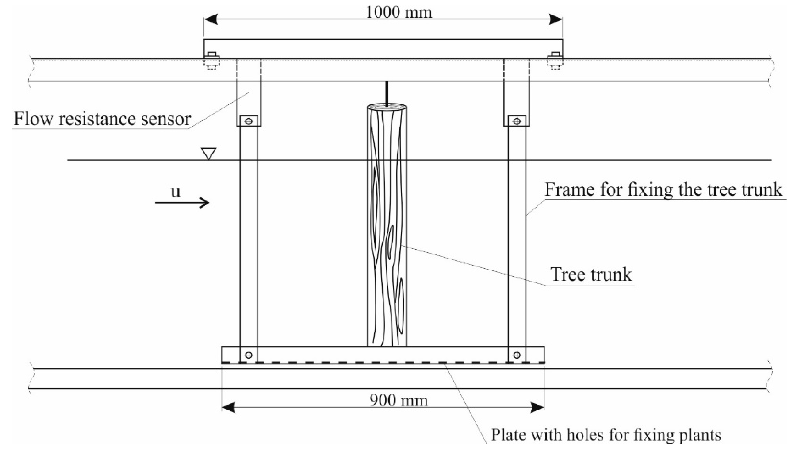
2.5. Evaluation of the Effect of Tree Trunk Bark Structure on Flow Resistance

Measurements were carried out in a laboratory in a hydraulic trough with 12 m in length, 0.47 m in width, and 0.9 m in height. The trough was flooded with water in a closed system with the maximum flow rate of 120 L∙s⁻¹. The trough filling was controlled by a lid at one end of the trough. The measuring system was equipped with an electromagnetic flow meter and an electronic sensor of the water level. In the trough there was a dynamometric platform connected to a tensometric sensor capable of measuring tangential and stretching forces in the range up to 0.05 kN (Figure 3). Moreover, water temperature and speed of water reaching the tree trunk were measured using a micro ADV probe. Measurements were made for 11 different mean flow values from the range 0.1–0.7 m∙s⁻¹ for two variants of the experiment: for the natural trunks and for the trunks wrapped in foil. Each measurement was repeated twice.

The results were analyzed for a relationship between the coefficient of flow resistance of particular tree trunk samples and the parameters used for characterization of their surfaces: average slopes, standard deviations of the slopes, ratio of 2D to 3D area, and BHF.

3. Results

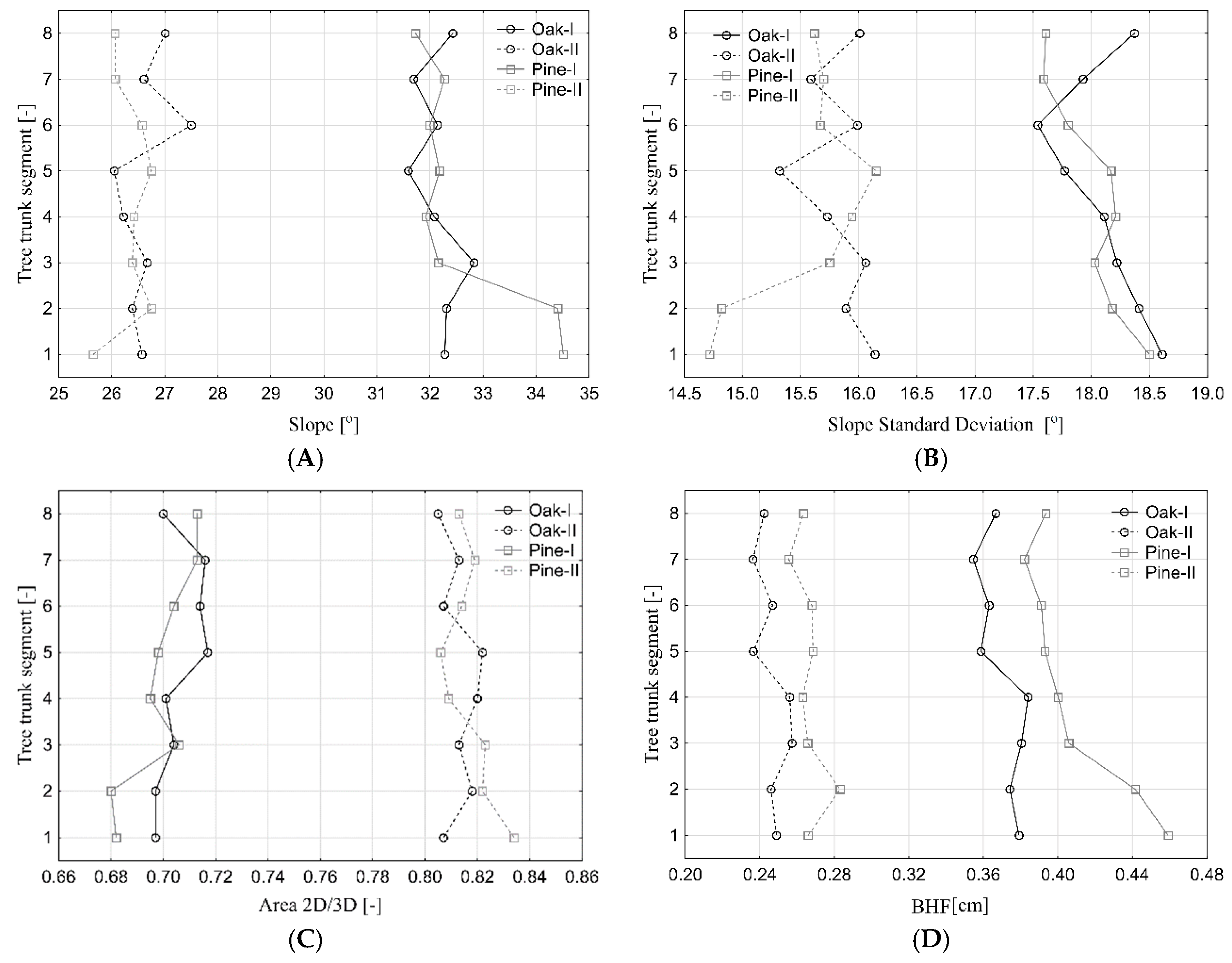
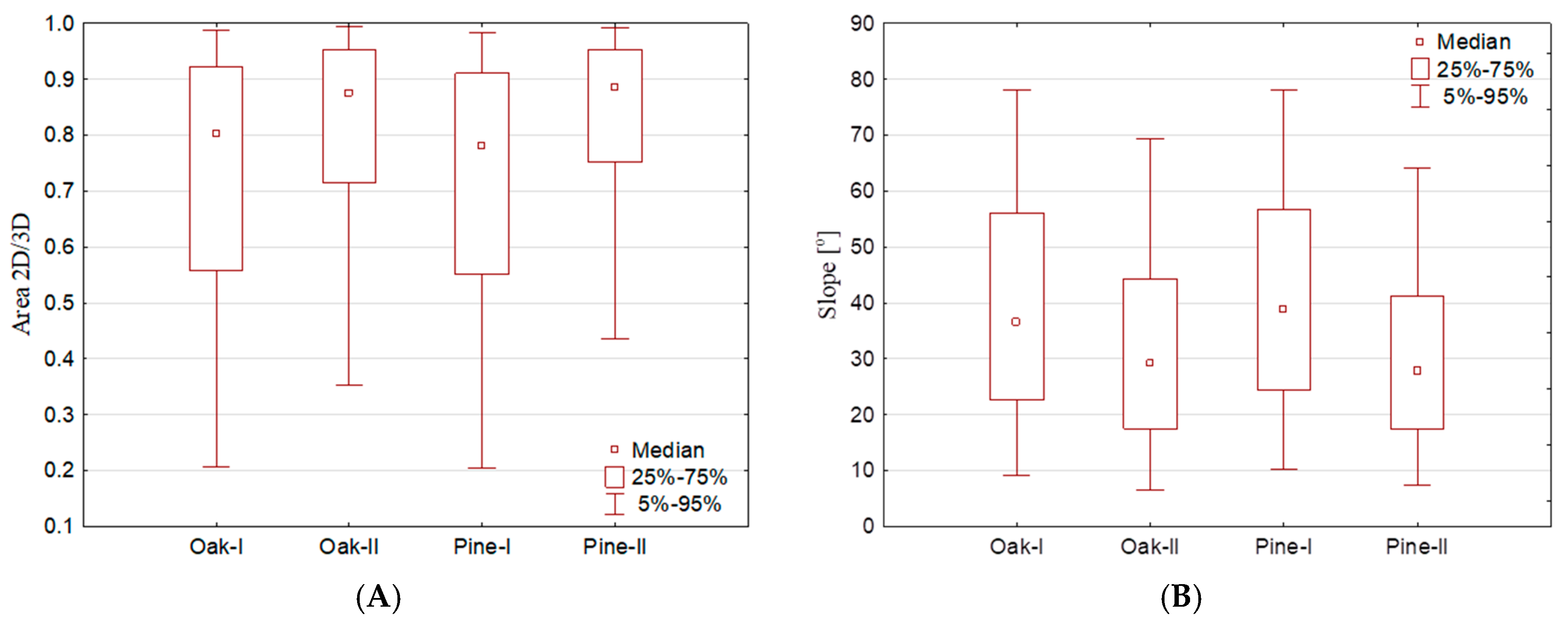
3.1. Bark Characteristics of Tree Trunks

The point clouds obtained from the scans made in laboratory conditions were combined into 3D models (Figure 4).

In the next step, using the TTBSM model, the point clouds were divided into segments 0.05 m in width, resulting in eight segments which were used in the analysis (Figure 5A). The transformed point clouds were the input data for generation of digital models of the tree trunk surfaces in the TIN format (Figure 5B). The use of the TIN model for the calculations followed from the necessity of preservation of the original data from the scans. Using the standard tools available in the ArcGIS environments, the average slope, standard deviation of slope, ratio of 2D to 3D area, and BHF (Figure 5C) were calculated.

Analysis of the surface sculpture of the natural tree trunks (Oak I, Pine I) and the foil-wrapped corresponding trunks (Oak II, Pine II) has shown the diversity of the surface structures (

Table 3. Characteristics of the surfaces of tree trunks studied.

		Slope (°)		Standard Deviation of Slope (°)		Area 2D/3D (-)		BHF (cm)
		Min	Mean	Min	Mean	Min	Mean	Min	Mean
		Max	Median	Max	Median	Max	Median	Max	Median
Oak	I	31.6	32.2	17.5	18.1	0.7	0.71	0.35	0.37
		32.8	32.1	18.6	18.1	0.72	0.7	0.38	0.37
	II	26.1	26.7	15.3	15.9	0.8	0.81	0.24	0.25
		27.5	26.6	16.2	16	0.82	0.81	0.26	0.25
Pine	I	31.7	32.6	17.6	18	0.68	0.7	0.38	0.41
		34.5	32.2	18.5	18	0.71	0.7	0.46	0.39
	II	25.7	26.4	14.7	15.7	0.79	0.81	0.26	0.27
		27.1	26.4	16.5	15.7	0.83	0.81	0.28	0.27

). The slopes measured for the natural tree trunks were higher than for the samples foil-wrapped and varied from 31.6 to 34.5° and 25.7 to 27.5°, respectively. For the oak and pine tree surfaces the average slopes were similar and equal to 32.2° and 32.6°, respectively. Lower roughness of the tree trunks foil-wrapped is also indicated by the analysis of average standard deviations equal to 15.7 and 15.9 for pine and oak tree trunks, respectively. The above results were confirmed by analysis of the ratio of 2D to 3D areas. For the natural tree trunks the average 2D to 3D area ratio was lower and close to 0.70, while for the trunks foil-wrapped this ratio was 0.81. Similarly, as for the slopes and their standard deviations, the ratios of 2D to 3D area of the trunks foil-wrapped were similar. For the natural tree trunks (without foil), the average BHF of the pine trunk was greater, 0.41 cm, while that of the oak trunk was 0.37 cm.

Analysis of bark structure characteristics of the foil-wrapped tree trunks, performed over segments of 0.05 m, revealed the greatest differences in the bottom parts of the trunks. The analysis indicate the greatest differences between the average slopes (Figure 6A) and 2D to 3D area ratios (Figure 6C) in segment no 1 and slope standard deviations in segments no 1, 2 and 5 (Figure 6B). The analysis of BHF for both foil-wrapped tree trunks indicate that for pine the values were slightly higher than in oak from 0.01 to 0.03 cm. The greatest differences were observed in segment no 2 (Figure 6D). The analysis of pine and oak trunks indicate the greatest differences between average slope, 2D to 3D area ratio and BHF were observed in their bottom segments no 1 and 2. The most uniform was the surface of the oak tree trunk, characterized over the whole length by the lowest variation in the slopes, 2D to 3D area ratios and BHF (Figure 6). For pine tree, the greatest BHF was noted in the bottom part of the trunk. The 2D to 3D area ratios for oak tree trunks proved that the difference between 2D and 3D area was up to 45% (percentile of 75%) for the natural tree trunk and 28% for the trunk wrapped in foil. For the pine tree the analogous difference was 48% and 26% for the natural and foil-wrapped trunk, respectively. For the tree trunks wrapped in foil, the 2D/3D area ratio in the percentile range 25–75% varied from 0.72 to 0.96, while for the natural trunks it varied from 0.55 to 0.93 (Figure 7A). The slope values in the percentile range 25–75% varied from 23 to 55° for the natural tree trunks, while for the foil-wrapped trunks the values were lower and varied from 17 to 43° (Figure 7B). The Kruskal–Wallis rank test indicate the statistical significant differences between medians of BHF and other bark characteristics for pine and oak natural and wrapped in foil trunks. Differences were significant at level of 0.05.

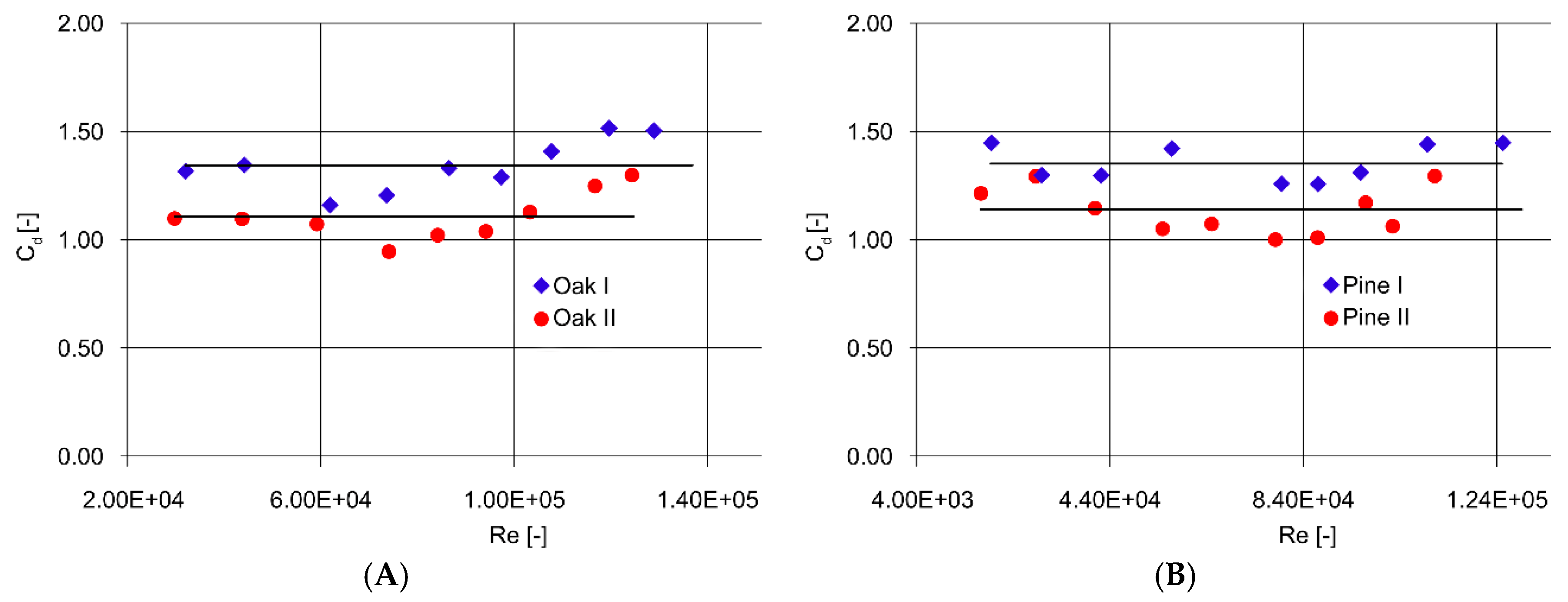
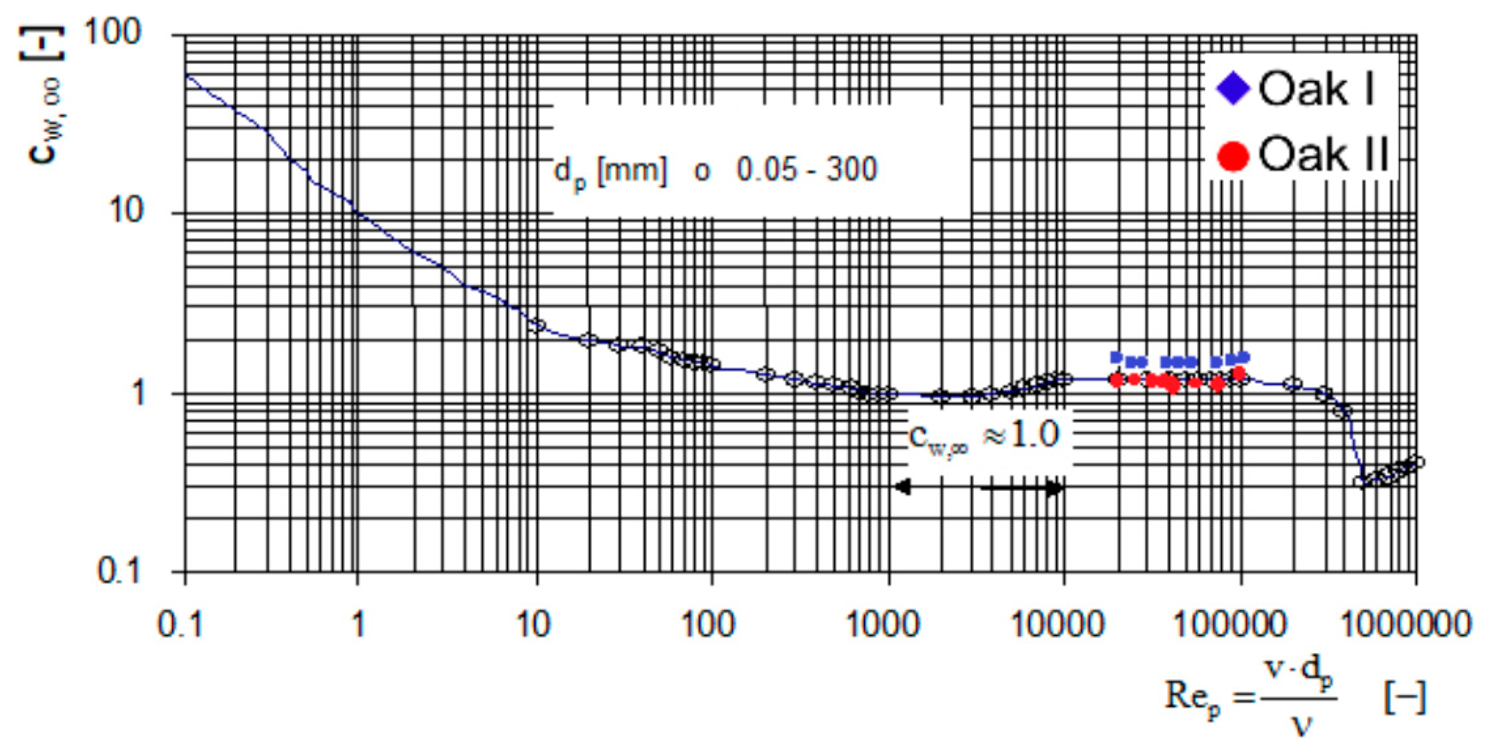
3.2. Relation between Flow Resistance of Trees and Bark Structure

On the basis of measurements performed in the hydraulic trough, the values of flow resistance coefficient Cd were calculated from Equation (3). The measured parameters included: resisting force on flow around a tree trunk $F_d$, tree trunk diameter $d_p$, depth of immersion h, speed of water approaching the tree trunk, and water temperature. The resisting force $F_d$ was calculated as the arithmetic mean from the results. The average tree trunk diameter dp was the mean value from diameter measurements at five heights of 0 m, 0.1 m, 0.2 m, 0.3 m, and 0.4 m. The depth of immersion h was the distance between the dynamometric plate on which the tree trunk was set and the water level measured using a micrometric pin. The speed of water approaching a tree trunk u was calculated as the mean value obtained in analysis of speed values distribution. The water temperature during the experiment was 18.10 °C. On the basis of the results of measurements substituted into Equation (2), the Reynolds number $R_e$ was found so that finally a relation between the flow resistance coefficient $C_d$ and the Reynolds number $R_e$ could be obtained. The values of resistance coefficient for variant I and II were averaged for the analyzed range of Reynolds number (horizontal lines in Figure 8). As follows from the results, for each tree species the flow resistance coefficient is greater for the natural trunk than for the trunk wrapped in foil (Figure 8).

The flow resistance coefficient calculated on the basis of average values is higher for the natural than for the foil-wrapped tree trunk, by about 22%. For $R_e$ > 10⁵ the values of the flow resistance coefficient increase for the natural trunk and that wrapped in foil to the values of 1.50 and 1.30, respectively. Mean value of $C_d$ for Oak I equals 1.35 and for Oak II 1.11. The bark structure of the natural oak tree trunk is responsible for the flow resistance coefficient increase by about 20% with respect to that for the trunk wrapped in foil. Similar results were obtained for Pine. The mean value of $C_d$ for Pine I equals 1.35 and for Pine II 1.13. In this case, the increase of BHF for natural tree trunk equals 20% (

Table 4. Comparison of results flow resistance coefficient $C_d$ for oak and pine.

Oak					Pine
${\mathit{R}}_{\mathit{e}}$	${\mathit{C}}_{\mathit{d}\mathit{I}}$	${\mathit{C}}_{\mathit{d}\mathit{I}\mathit{I}}$	$\Delta {\mathit{C}}_{\mathit{d}}$	%	${\mathit{R}}_{\mathit{e}}$	${\mathit{C}}_{\mathit{d}\mathit{I}}$	${\mathit{C}}_{\mathit{d}\mathit{I}\mathit{I}}$	$\Delta {\mathit{C}}_{\mathit{d}}$	%
3.19 × 104	1.32	1.10	0.22	20	1.71 × 104	1.44	1.21	0.24	20
4.42 × 104	1.35	1.10	0.25	23	2.84 × 104	1.30	1.29	0.01	1
6.17 × 104	1.16	1.07	0.09	8	4.08 × 104	1.30	1.14	0.16	14
7.34 × 104	1.21	0.95	0.26	28	5.47 × 104	1.42	1.05	0.37	35
8.64 × 104	1.33	1.03	0.31	30	6.48 × 104	1.30	1.07	0.23	21
9.71 × 104	1.30	1.04	0.26	25	7.80 × 104	1.26	1.00	0.26	26
1.08 × 105	1.41	1.13	0.28	25	8.65 × 104	1.26	1.01	0.25	25
1.20 × 105	1.52	1.25	0.27	22	9.66 × 104	1.31	1.17	0.15	12
1.37 × 105	1.52	1.30	0.22	17	1.02 × 105	1.44	1.06	0.38	35
1.29 × 105	1.51	1.29	0.22	17	1.11 × 105	1.45	1.29	0.16	12

). The largest absolute differences between the values of $C_d$ occurred in the case of pine and amounted to 0.38. Table 4 also presents the percentage increase in $C_d$ for the natural stem related to foil wrapped.

4. Discussion

An increase in knowledge about simple and complex canopy roughness for various types of vegetation is necessary, especially when considering overall roughness inputs in hydraulic modeling. The study conducted by Antonarakis et al. [28] aimed to determine stem roughness friction factors for the below-canopy flow; for this reason they used such parameters of trees as trunk location, height, and diameter. Total height-derived trunk diameters using the tree detection and crown segmentation (TDCS) method produced the closest roughness coefficient values to the ground-derived roughness coefficients. The stem roughness values produced from this method fell within guideline values. Studies performed to date on the use of TLS have mainly concerned the 3D bark texture analysis and have been used for identification of tree species [27,30,36,37]. The results of this study have shown the potential of GIS tools and TLS data for analysis of bark structure characteristics of tree trunks in floodplains. In particular, high resolution of the point clouds permits advanced analyses, including that of the tree trunk texture. The possibility to determine the bark structure characteristics supplements the already proven applications of TLS demonstrated by Kankare et al. [34] and Hyyti and Visala [35], for determination of the diameter at breast height (DBH), tree heights, wood volume, tree stem ovality, structure and damage of bark, tree topology, and branch angles and diameters. Determination of the bark structure characteristics of trees permits a more accurate evaluation of the roughness coefficients of floodplains. As demonstrated by Antonarakis et al. [16], tree trunks are major contributors to roughness in a densely wooded floodplain. The proposed method for determination of bark structure characteristics can be used in the field, and meets the requirements defined by Tanaka et al. [19], according to which the measurement of canopy structure must be nondestructive.

Dassot et al. [45] and Kükenbrink et al. [46] have shown that evaluation of the flow resistance of vegetation requires the millimeter resolution. The use of ALS data in this case is impossible [48]. Only the use of TLS measurements permits construction of high-resolution models of tree trunks and their parametrization (determination of the bark structure characteristics and their changes along the tree trunk). According to Tanaka et al. [44], it is very important to determine the drag characteristics of real tree trunks with various barks. The developed Tree Trunk Bark Structure Model can be commonly used for all tree species. This research also demonstrates the ability of terrestrial scanning in ideal laboratory conditions to extract meaningful information about the tree trunk. To estimate bark structure characteristics of the tree trunk in the field, optimal scanning conditions must be ensured. During the laboratory measurements there were ideal conditions for scanning and the distance from the scanner to the tree trunks was up to 2.5 m. Locating the scanner at a greater distance while maintaining the same scan quality may only allow for determining the location of individual trees and estimating the trunk diameter. As Brolly and Király [27] suggested, the tree diameters determined on the basis of laser scanning may be different than the real ones, especially in the case of rough barked and noncircular stem cross-section trees. The methodology presented in this study should be verified in the field on different tree species with varying age. According to Othmani et al. [36], it will help to standardize the tree to a scanner distance that has an impact on the resolution of the point cloud in order to obtain point clouds of sufficiently good resolution in a reasonable time. Othmani et al. [30] demonstrated that scanning a tree with a diameter of about 30 cm with a TLS at 6 m allows for the analysis of the 3D geometric texture of the bark in order to compute roughness measures and shape characteristics. The methods presented in this study may have limitations in in situ measurement, with the first being the quality of the scanner data. Antonarakis et al. [26] suggested that the issue with the methods derived from the ground scanning data was a combination of two factors. The first was the effect of the wind on the scanning of the objects, and the second was the points reflected from the edges of objects. Another factor that may influence the result of the proposed method in the field is, according to Brolly and Király [27], to assure optimal conditions for scanning the leaf-off state, the lack of shrubs, the high crown bases, and the moderate terrain variability.

Our results showed that the tree trunk bark structure increases the flow resistance of trees by about 20% compared to tree trunks wrapped in foil. It should be stated that these are preliminary results, based only on two tree trunks, which can only show that bark structure impact in hydraulic modeling should not be neglected. The presented methodology may be useful for the study of different trees of the same and different species in order to determine the impact of bark structure on the flow resistance coefficient more accurately. The universal character of the method proposed means that it can be applied in a wider range, defined by Tanaka et al. [44], for analysis of vertical stand structure of trunk and branches.

The experimentally determined coefficients of flow resistance for the tree trunks wrapped in foil take values similar to that obtained by Schlichting and Gersten [49], which was $C_d$ = 1.1, for smooth tree trunks for the Reynolds number 3·10⁴ < $R_e$ < 10⁵ (Figure 9 and Figure 10). The natural trunks, both oak and pine, achieved larger values of $C_d$. This shows that not taking into account the bark characteristics may lead to underestimating of $C_d$ and further on lowering the value of friction factor (Equation (1)). The figures also show that the conducted research covers only on certain range of $R_e$ values. However, it is particularly interesting from the point of view of average conditions occurring during floods when water may flow in areas covered with trees (velocities 0.1–0.5 m/s).

In the same paper [49], it was assumed that the contribution of the tree trunk roughness to the total flow resistance of a smooth cylinder is 11%, so it can be neglected; however, the laboratory tests performed by us indicated that this contribution is much greater and reaches 20%. Similar results were obtained by Ruck et al. [50], who studied the flow around the cylinder with increased roughness. The used roughness varied according to the layer thickness of balls coated on the cylinder. Three different layer thicknesses were tested: 3, 5, and 10 mm. For both experimental series, the Reynolds number was systematically varied in the range from 1.0·10⁴ to 1.3∙10⁵. The drag coefficients obtained in research seem to be quite constant in the investigated range of Reynolds numbers. The drag coefficients of the fully coated cylinders are 15–25% higher than for the smooth cylinder. Obviously, the drag increases with increasing layer thickness. Values obtained in our research for natural stems were similar for BHF ranging from 3 to 10 mm. This confirmed the importance of this parameter on the coefficient of resistance to the flow of tree trunks.

5. Conclusions

The overall scope of this modeling exercise was to illustrate the effects of tree trunk bark structure on flow resistance coefficient. This was achieved by comparing a natural and foil-wrapped tree trunk. A combination of the capabilities of GIS tools and TLS technique offers great possibilities of advanced measurements and analyses. Terrestrial laser scanning has been used in this study to define tree trunk bark at a millimeter resolution for the purpose of parameterizing bark structure in resistance equations.

The presented method of TLS scanning resulted in a high resolution of the point clouds, reaching 50 points/cm², which allows for the development of highly detailed 3D models that can be used for analyzing tree trunk structure. The developed TTBSM model allows one to automate the process of calculating the bark characteristics of tree trunks based on the TLS data. The model can be used to analyze various species of trees of different ages.

For the natural tree trunks, the average BHF of the pine trunk was greater, 0.41 cm, while that of the oak trunk was 0.37 cm. As follows from the analysis of bark structure characteristics of tree trunks along their length, the variation of this parameter was observed. The analysis of pine and oak trunks indicates the greatest differences between average slope, 2D to 3D area ratio and BHF in the bottom part. The surface of the oak tree trunk was most uniform and was characterized by the lowest spatial variation of slopes, 2D to 3D area ratios and roughness. Analysis of BHF parameters of the foil-wrapped tree trunks, performed over segments of 0.05 m, indicate that for pine the values were slightly higher than in oak, from 0.01 to 0.03 cm.

The results presented and discussed above have proved that the bark structure of tree trunks has a significant impact on the flow resistance of trees. For the pine and oak tree trunks studied, the coefficient of flow resistance $C_d$ for the natural trunks was on average 20% higher than that for the trunks wrapped in foil. We have shown that the impact of the tree trunk bark structure analyzed with respect to the impact of the shape of the body (cylinder) on the coefficient of flow resistance $C_d$ is greater than it has been hitherto assumed on the basis of literature data. The ratio of 20 to 80% is significantly different than the literature ratio of 10 to 90%. In view of that, the assumption that the effect of bark structure of tree trunks can be neglected is unfounded and can lead to a considerable error in the evaluation of flow conditions in forested floodplains.

References

1. Baptist, M.J.; Babovic, V.; Rodríguez Uthurburu, J.; Keijzer, M.; Uittenbogaard, R.E.; Mynett, A.; Verwey, A. On inducing equations for vegetation resistance. J. Hydraul. Res. 2007, 45, 435–450. [Google Scholar] [CrossRef]
2. Horritt, M.S. A methodology for the validation of uncertain flood inundation models. J. Hydrol. 2006, 326, 153–165. [Google Scholar] [CrossRef]
3. Klopstra, D.; Barneveld, H.J.; van Noortwijk, J.; van Velzen, E. Analytical model for hydraulic roughness of submerged vegetation. In Proceedings of the 27th IAHR Conference, San Francisco, CA, USA, 10–15 August 1997; American Society of Civil Engineers (ASCE): New York, NY, USA, 1997; pp. 775–780. [Google Scholar]
4. Wu, Y.; Falconer, R.A.; Struve, J. Mathematical modelling of tidal currents in mangrove forests. Environ. Model. Softw. 2001, 16, 19–29. [Google Scholar] [CrossRef]
5. Yang, W.; Choi, S.U. A two-layer approach for depth-limited open-channel flows with submerged vegetation. J. Hydraul. Res. 2010, 48, 466–475. [Google Scholar] [CrossRef]
6. Crosato, A.; Saleh, M.S. Numerical study on the effects of floodplain vegetation on river planform style. Earth Surf. Proc. Landf. 2011, 36, 711–720. [Google Scholar] [CrossRef]
7. Perona, P.; Camporeale, C.; Perucca, E.; Savina, M.; Molnar, P.; Burlando, P.; Ridolfi, L. Modelling river and riparian vegetation interactions and related importance for sustainable ecosystem management. Aquat. Sci. 2009, 71, 266. [Google Scholar] [CrossRef]
8. Velasco, D.; Bateman, A.; Medina, V. A new integrated, hydro-mechanical model applied to flexible vegetation in riverbeds. J. Hydraul. Res. 2008, 46, 579–597. [Google Scholar] [CrossRef]
9. Meijer, D.G.; Van Velzen, E.H. Prototype-scale flume experiments on hydraulic roughness of submerged vegetation. In Proceedings of the 28th International IAHR Conference, Graz, Austria, 22–27 August 1999; Technical University Graz, Institute for Hydraulics and Hydrology: Graz, Austria, 1999. [Google Scholar]
10. Murphy, E.; Ghisalberti, M.; Nepf, H. Model and laboratory study of dispersion in flows with submerged vegetation. Water Resour. Res. 2007, 43. [Google Scholar] [CrossRef] [Green Version]
11. Tal, M.; Paola, C. Effects of vegetation on channel morphodynamics: Results and insights from laboratory experiments. Earth Surf. Proc. Landf. 2010, 35, 1014–1028. [Google Scholar] [CrossRef]
12. Straatsma, M. 3D float tracking: In situ floodplain roughness estimation. Hydrol. Process. 2009, 23, 201–212. [Google Scholar] [CrossRef]
13. Walczak, Z.; Sojka, M.; Wróżyński, R.; Laks, I. Estimation of Polder Retention Capacity Based on ASTER, SRTM and LIDAR DEMs: The Case of Majdany Polder (West Poland). Water 2016, 8, 230. [Google Scholar] [CrossRef]
14. Laks, I.; Sojka, M.; Walczak, Z.; Wróżyński, R. Possibilities of Using Low Quality Digital Elevation Models of Floodplains in Hydraulic Numerical Models. Water 2017, 9, 283. [Google Scholar] [CrossRef]
15. Forzieri, G.; Degetto, M.; Righetti, M.; Castelli, F.; Preti, F. Satellite multispectral data for improved floodplain roughness modelling. J. Hydrol. 2011, 407, 41–57. [Google Scholar] [CrossRef]
16. Antonarakis, A.S.; Richards, K.S.; Brasington, J.; Muller, E. Determining leaf area index and leafy tree roughness using terrestrial laser scanning. Water Resour. Res. 2010, 46. [Google Scholar] [CrossRef] [Green Version]
17. Petryk, S.; Bosmajian, G., III. Analysis of flow through vegetation. J. Hydraul. Div. 1975, 101, 871–884. [Google Scholar]
18. Arcement, G.J.; Schneider, V.R. Guide for Selecting Manning’s Roughness Coefficients for Natural Channels and Flood Plains; U.S. Geological Survey: Denver, CO, USA, 1989.
19. Tanaka, T.; Yamaguchi, J.; Takeda, Y. Measurement of forest canopy structure with a laser plane range-finding method—Development of a measurement system and applications to real forests. Agric. For. Meteorol. 1998, 91, 149–160. [Google Scholar] [CrossRef]
20. Lindner, K. Der Strömungswiderstand von Pflanzenbeständen; Mitteilungen; Heft 75; Technische Universität Braunschweig; Leichtweiss-InstitutfürWasserbau: Braunschweig, Germany, 1982. [Google Scholar]
21. Nakayama, A. Introduction to Fluid Mechanics; Butterworth-Heinemann: Oxford, UK, 1999. [Google Scholar]
22. Aberle, J.; Järvelä, J. Flow resistance of emergent rigid and flexible floodplain vegetation. J. Hydraul. Res. 2013, 51, 33–45. [Google Scholar] [CrossRef]
23. Straatsma, M.W.; Baptist, M.J. Floodplain roughness parameterization using airborne laser scanning and spectral remote sensing. Remote Sens. Environ. 2008, 112, 1062–1080. [Google Scholar] [CrossRef]
24. Casas, A.; Lane, S.N.; Yu, D.; Benito, G. A method for parameterising roughness and topographic sub-grid scale effects in hydraulic modelling from LiDAR data. Hydrol. Earth Syst. Sci. 2010, 14, 1567–1579. [Google Scholar] [CrossRef] [Green Version]
25. Shendryk, I.; Broich, M.; Tulbure, M.G.; Alexandrov, S.V. Bottom-up delineation of individual trees from full-waveform airborne laser scans in a structurally complex eucalypt forest. Remote Sens. Environ. 2016, 173, 69–83. [Google Scholar] [CrossRef]
26. Antonarakis, A.S.; Richards, K.S.; Brasington, J.; Bithell, M. Leafless roughness of complex tree morphology using terrestrial lidar. Water Resour. Res. 2009, 45. [Google Scholar] [CrossRef] [Green Version]
27. Brolly, G.; Király, G. Algorithms for stem mapping by means of terrestrial laser scanning. Acta Silvatica et Lignaria Hungarica 2009, 5, 119–130. [Google Scholar]
28. Antonarakis, A.S.; Richards, K.S.; Brasington, J.; Bithell, M.; Muller, E. Retrieval of vegetative fluid resistance terms for rigid stems using airborne lidar. J. Geophys. Res. Biogeosci. 2008, 113. [Google Scholar] [CrossRef] [Green Version]
29. Lovell, J.L.; Jupp, D.L.B.; Newnham, G.J.; Culvenor, D.S. Measuring tree stem diameters using intensity profiles from ground-based scanning lidar from a fixed viewpoint. ISPRS J. Photogramm. Remote Sens. 2011, 66, 46–55. [Google Scholar] [CrossRef]
30. Othmani, A.; Piboule, A.; Dalmau, O.; Lomenie, N.; Mokrani, S.; Voon, Y. Tree species classification based on 3D bark texture analysis. In Proceedings of the Pacific-Rim Symposium on Image and Video Technology; Springer: Berlin, Germany, 2013; pp. 279–289. [Google Scholar]
31. Bienert, A.; Maas, H.G.; Scheller, S. Analysis of the information content of terrestrial laser scanner point clouds for the automatic determination of forest inventory parameters. In Proceedings of the Workshop on 3D Remote Sensing in Forestry, Vienna, Austria, 14–15 February 2006; Volume 14, pp. 1–7. [Google Scholar]
32. Yang, X.; Strahler, A.H.; Schaaf, C.B.; Jupp, D.L.; Yao, T.; Zhao, F.; Dubayah, R.O. Three-dimensional forest reconstruction and structural parameter retrievals using a terrestrial full-waveform lidar instrument (Echidna®). Remote Sens. Environ. 2013, 135, 36–51. [Google Scholar] [CrossRef]
33. Wang, D.; Hollaus, M.; Puttonen, E.; Pfeifer, N. Fast and robust stem reconstruction in complex environments using terrestrial laser scanning. Int. Arch. Photogramm. Remote Sens. Spat. Inf. Sci. 2016, 41, 411–417. [Google Scholar] [CrossRef]
34. Kankare, V.; Holopainen, M.; Vastaranta, M.; Puttonen, E.; Yu, X.; Hyyppä, J.; Alho, P. Individual tree biomass estimation using terrestrial laser scanning. ISPRS J. Photogramm. Remote Sens. 2013, 75, 64–75. [Google Scholar] [CrossRef]
35. Hyyti, H.; Visala, A. Feature Based modeling and mapping of tree trunks and natural terrain using 3D laser scanner measurement system. IFAC Proc. Vol. 2013, 46, 248–255. [Google Scholar] [CrossRef]
36. Othmani, A.A.; Jiang, C.; Lomenie, N.; Favreau, J.M.; Piboule, A.; Voon, Y. A novel computer-aided tree species identification method based on burst wind segmentation of 3D bark textures. Mach. Vis. Appl. 2016, 27, 751–766. [Google Scholar] [CrossRef]
37. Lin, Y.; Herold, M. Tree species classification based on explicit tree structure feature parameters derived from static terrestrial laser scanning data. Agric. For. Meteorol. 2016, 216, 105–114. [Google Scholar] [CrossRef]
38. Hosoi, F.; Omasa, K. Voxel-based 3-D modeling of individual trees for estimating leaf area density using high-resolution portable scanning lidar. IEEE Trans. Geosci. Remote Sens. 2006, 44, 3610–3618. [Google Scholar] [CrossRef]
39. Calders, K.; Armston, J.; Newnham, G.; Herold, M.; Goodwin, N. Implications of sensor configuration and topography on vertical plant profiles derived from terrestrial LiDAR. Agric. For. Meteorol. 2014, 194, 104–117. [Google Scholar] [CrossRef]
40. Calders, K.; Newnham, G.; Burt, A.; Murphy, S.; Raumonen, P.; Herold, M.; Kaasalainen, M. Nondestructive estimates of above-ground biomass using terrestrial laser scanning. Methods Ecol. Evol. 2015, 6, 198–208. [Google Scholar] [CrossRef]
41. Sioma, A.; Socha, J.; Klamerus-Iwan, A. A New Method for Characterizing Bark Microrelief Using 3D Vision Systems. Forests 2018, 9, 30. [Google Scholar] [CrossRef]
42. Westoby, M.J.; Brasington, J.; Glasser, N.F.; Hambrey, M.J.; Reynolds, J.M. ‘Structure-from-Motion’ photogrammetry: A low-cost, effective tool for geoscience applications. Geomorphology 2012, 179, 300–314. [Google Scholar] [CrossRef] [Green Version]
43. Wróżyński, R.; Pyszny, K.; Sojka, M.; Przybyła, C.; Murat-Błażejewska, S. Ground volume assessment using ‘Structure from Motion’ photogrammetry with a smartphone and a compact camera. Open Geosci. 2017, 9, 281–294. [Google Scholar] [CrossRef]
44. Tanaka, N.; Takenaka, H.; Yagisawa, J.; Morinaga, T. Estimation of drag coefficient of a real tree considering the vertical stand structure of trunk, branches, and leaves. Int. J. River Basin Manag. 2011, 9, 221–230. [Google Scholar] [CrossRef]
45. Dassot, M.; Colin, A.; Santenoise, P.; Fournier, M.; Constant, T. Terrestrial laser scanning for measuring the solid wood volume, including branches, of adult standing trees in the forest environment. Comput. Electron. Agric. 2012, 89, 86–93. [Google Scholar] [CrossRef]
46. Kükenbrink, D.; Schneider, F.D.; Leiterer, R.; Schaepman, M.E.; Morsdorf, F. Quantification of hidden canopy volume of airborne laser scanning data using a voxel traversal algorithm. Remote Sens. Environ. 2017, 194, 424–436. [Google Scholar] [CrossRef]
47. ASME. Surface Texture (Surface Roughness, Waviness, and Lay): An American Standard; ASME B46.1-1995 (Revision of ANSI/ASME B46.1-1985); ASME: New York, NY, USA, 1996. [Google Scholar]
48. Walczak, Z.; Sojka, M.; Laks, I. Assessment of mapping of embankments and control structure on digital elevation model based up on Majdany polder. Rocznik Ochrona Srodowiska 2013, 15, 2711–2724. [Google Scholar]
49. Schlichting, H.; Gersten, K. Grenzschicht-Theorie; Springer: Berlin/Heidelberg, Germany, 2006. [Google Scholar]
50. Ruck, B.; Klausmann, K.; Wacker, T. Drag reduction of cylinders by partial porous coating. In Proceedings of the 9th International Conference on Heat Transfer, Fluid Mechanics and Thermodynamics, Malta, 16–18 July 2012. [Google Scholar]
Figure 1. Scan of the trunk (P) with the four reference balls (K); photogrammetric image of point cloud intensity.
Water 10 00753 g001
Figure 2. The scheme of TTBSM processing.
Water 10 00753 g002
Figure 3. Scheme of the measuring setup and view of the hydraulic trough.
Water 10 00753 g003
Figure 4. Example of 3D model of the oak tree trunk, (A) wrapped in foil; (B) natural.
Water 10 00753 g004
Figure 5. (A) transformed point cloud; (B) triangulated irregular network; (C) Bark height factor (BHF) of Oak I and Oak II samples.
Water 10 00753 g005
Figure 6. Changes in the slope (A); standard deviation of slope (B); 2D to 3D area ratio (C) and BHF (D) along the trunks of oak and pine trees.
Water 10 00753 g006
Figure 7. Statistical analysis of 2D/3D area ratio (A) and slope (B) for oak and pine tree trunks.
Water 10 00753 g007
Figure 8. Flow resistance coefficient C d versus Reynolds number Re for oak (A) and pine (B).
Water 10 00753 g008
Figure 9. Flow resistance coefficient C d versus Reynolds number R e for oak against the C d = f ( R e ) [49].
Water 10 00753 g009
Figure 10. Flow resistance coefficient C d versus Reynolds number Re for pine against the C d = f ( R e ) [49].
Water 10 00753 g010