Decision Support for the Design and Operation of Variable Speed Pumps in Water Supply Systems
by
 ,
,
Dimitri Nowak
1,* ,
,
Helene Krieg
1,
Michael Bortz
1,
Christian Geil
2,
Axel Knapp
2,
Harald Roclawski
2 and
Martin Böhle
2 1
Fraunhofer Institute ITWM, 67663 Kaiserslautern, Germany
2
Department of Mechanical Engineering, Institute for Turbomachinery and Fluid Mechanics, University of Kaiserslautern, 67663 Kaiserslautern, Germany
*
Author to whom correspondence should be addressed.
Water 2018, 10(6), 734; https://doi.org/10.3390/w10060734
Submission received: 29 March 2018
/
Revised: 18 May 2018
/
Accepted: 30 May 2018
/
Published: 5 June 2018
(This article belongs to the Special Issue Energy Efficient Management of Water Collection, Treatment, Storage and Distribution)
Abstract
:The design and operation of water supply systems is a multicriteria task: the energy efficiency should be minimized while, at the same time, respecting technical requirements, such as the balanced operation of available pumps. On one hand, the overall system can be improved by the use of variable speed pumps. They increase the number of operating options. On the other hand, they add more complexity to the operation problem. In this paper, we discuss the difficulties associated with speed control and propose a decision support process to overcome them.
1. Introduction
The optimization of water distribution systems is an important task to ensure the supply of drinking water is of excellent quality at acceptable cost for the population while taking into account the sustainability of water resources. It plays an important role in industry, for operators of water supply systems and in the scientific community. A recent review of scientific papers published since the 1980s was published by Mala-Jetmarova in [1]. It shows that there are various application areas for the optimization of water distribution systems. In [1], the papers are categorized into Design, Strengthening, Expansion, Rehabilitation and Operation. Among the elements of the water distribution system, which are optimized, one can distinguish between pipes, tanks, pumps and valves.
In any water supply system, the pumping of drinking water produces substantial energy costs resulting from the operation of pumps. In Germany, an average of 0.51 kWh is necessary to provide 1000 L of drinking water [2]. According to Grundfoss, one of the worlds largest pump manufacturers, for two thirds of the currently operated pumps, energy savings of up to 60% are possible [3]. Therefore, the focus of this paper is the optimization of pump operation in already existing water distribution systems. The current state-of-the-art system for this case is also described in detail in [1]. It is described that there are three optimization variables for pumps: the location, the size of the pump and the pump schedule. These variables have different impacts on the optimization method and require different algorithms. Until now, it has not been clear which algorithm is the best for a specific task. In [4], different approaches for improving the efficiency of a water supply network are reviewed. The literature is separated into two types of pump control optimization problems. The most common problems deal with constant speed pumps and less common problems consider variable speed pumps. Nevertheless, the conclusion drawn is that the installation of variable speed drives in pumps combined with control optimization may provide the greatest reduction in energy and costs associated with the network operation. For water systems equipped with variable speed pumps, according to [5], it may be possible to save up to of energy by a decrease in pump speed. However, the use of variable speed drives significantly increases the search space as well as the complexity of the optimization problem [1,6]. They introduce continuous parameters to the operation problem that can no longer be enumerated. Also, an algorithm has to take into account maintenance requirements and unpredictable events, like pump failure, when calculating an optimized pump schedule.
In this paper, we present a method for the calculation of Pareto optimal pump schedules for already existing water distribution systems, taking into account variable speed drives. This method can also be used for choosing an optimal pump size. It provides decision support to operators of water distribution systems.
In water supply system engineering, there are many different approaches for the provision of decision support [7]. For example, in [8], a Honey Bees Mating Optimization Algorithm was used to optimize pump schedules for four pumping stations, three tanks and a constant level water source using a simplified model of the piping network. In many cases, evolutionary algorithms have been used to solve the pump scheduling problem in combination with meta-models [9] or numerical models of the distribution network (e.g., [10,11,12]). In [13], the problem of optimizing pump scheduling was defined as a mixed integer problem and solved by the branch and bound method. The impacts of different approximations of system components and their effects on the loss in accuracy as well as on computational cost were investigated. We propose a different approach. Instead of integrating all user information into a single objective optimization problem, as proposed in [13], for example, we solve the entire multicriteria optimization problem (MOP), i.e., any solution for the weighted sum formulation of the MOP is represented in the solution set of the MOP since any optimal solution to a weighted sum problem is also Pareto optimal [14]. Consequently, instead of presenting the user with a single solution, the user is supported in the investigation of the best alternative (Pareto optimal [15]) solutions which perform better in some objectives at the cost of performance in other objectives. The idea of traversing the solution tree in this process is branch and bound [16]. However, cutting off branches of dominated solutions is processed in terms of a multicriteria comparison. This multicriteria approach is the main difference from many preexisting approaches.
In this paper, we continue our work [17] on an assistance software for local drinking water suppliers in medium size cities (approximately 100,000 inhabitants). The purpose of the software is to assist German drinking water supply companies in the management of their waterworks systems, that is to say, the operation and selection of new pumps. The emphasis in this paper is on the management of variable speed pumps.
It is of great importance to understand both the operation problem and the selection problem as multicriteria optimization problems. For both problems, the highest priority is the goal of satisfying the demand for drinking water. However, other criteria, such as the energy consumption or pump wear, may be difficult to weight up. Furthermore, there are technical requirements, such as water exchange in the tank, to sustain a certain drinking water quality. In addition, some factors are rather circumstantial, such as unscheduled maintenance. All this input is taken into account by the prototype developed at the Fraunhofer Institute for Industrial Mathematics ITWM in collaboration with the Institute for Fluid Mechanics and Turbomachinery of the Technical University in Kaiserslautern. In accordance with our previous work, the operator is involved into the decision process [17].
The question that will be answered is: How can speed control be efficiently integrated into our current MOP approach?
First, the computational complexity is addressed. If the operator decides to consider a finite number of speed control values, then, the number of alternative operation states will increase exponentially and, thus, dramatically slow down the solution generating process. Therefore, the operator has access to a limited number of speed control values. The operation problem stays discrete and can be treated analogously to our work in [17]. It is much more interesting to consider a range of speed control values. Then, the operation problem in every time step of a one-day cycle can be solved in terms of a nonlinear multivariate optimization problem. This way the exponential increase is prevented, but, we have to apply more sophisticated gradient methods [18]. The optimization process is discussed in Section 5 in more detail.
Second, the decision support process is addressed in Section 6. The operator can use the interactive tool from [17] to compare and modify decisions. Additionally, the operator is supported to evaluate certain speed control options to make sure that a pump is suitable for daily use.
Finally, we examine a single tank with multiple pumps system in Section 7 with respect to speed control. The operation problem is solved for different instances of technical requirement. For the selection problem, variable speed pumps are compared with respect to energy savings.
2. Model
To demonstrate our optimization method, we use a simplified, yet realistic, model of a well known water supply system which has already been presented in [17]. In Germany, it can be applied to various communities. The main idea of the model was to describe the piping system in terms of a characteristic curve. Depending on the drinking water consumption and the drinking water storage, the system curve adjusts. Intersecting the system curve with the characteristic curve of a pump yields an operation point. For more complex systems, hydraulic models must be modeled in more detail with EPANET. The EPANET model can then be coupled with our optimization method. Based on the daily drinking water demand and the choice of operating pumps, we can simulate an operation schedule for the waterworks and evaluate it with respect to target functions, which represent the individual preferences of the operator. Given that is the number of pumps, is the number of operating time steps and is the number of objectives, we face the following operation problem:
where s denotes an operation schedule, and f denotes the objective function vector of personal preferences, such as the energy efficiency or small number of pump switches. The constraint function g represents technical operating requirements, e.g., the limited capacity of the water storage. The amount of stored drinking water is limited by the minimal capacity due to safety regulations and must not exceed the maximal capacity of the containers to prevent an overflow. Let S be the set of allowed operating schedules. For the operation problem, the pumps are allowed to operate in parallel with no speed control,
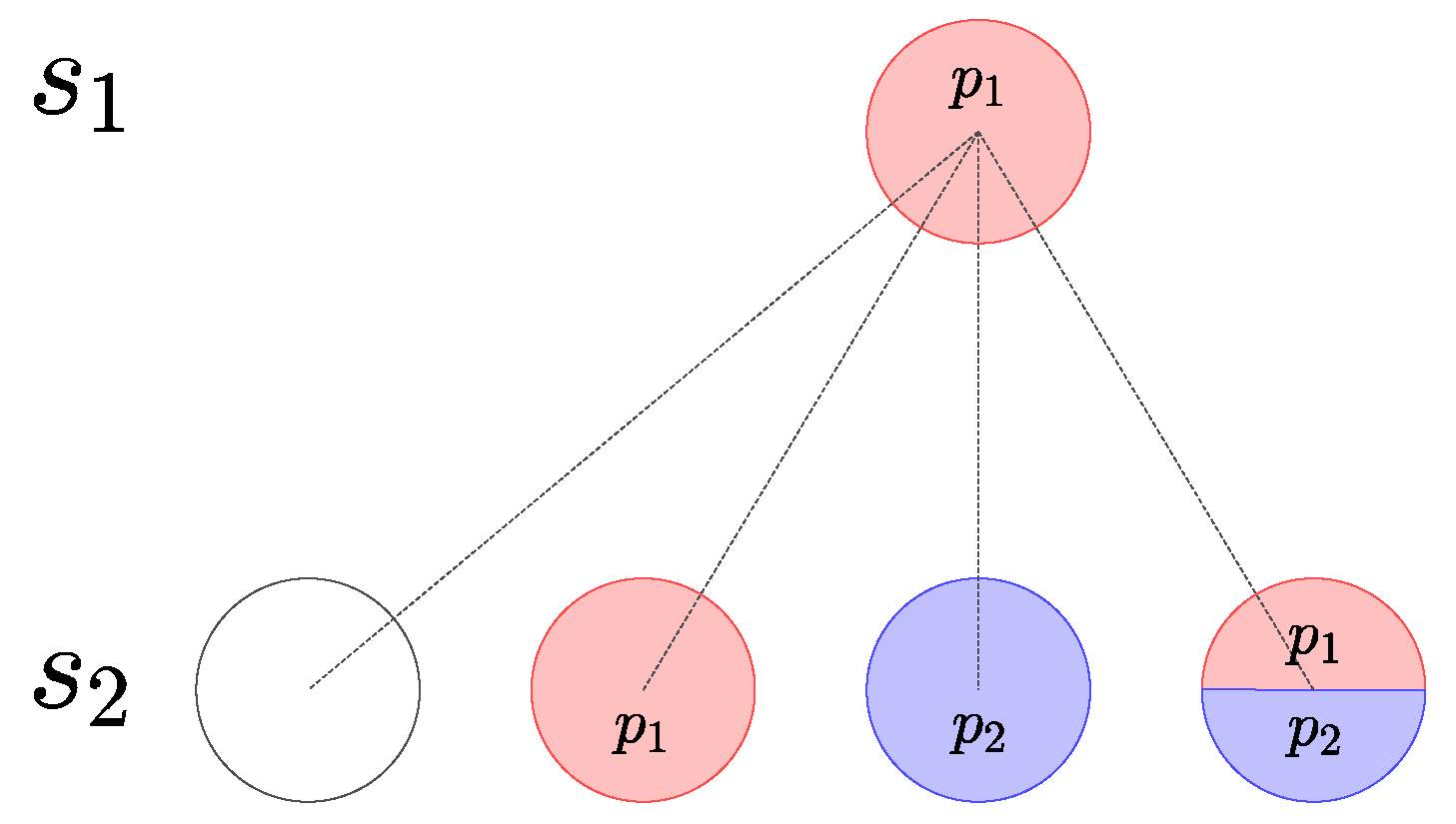
where denotes the power set of a set, i.e., each subset of pumps can be used for operation: no pump, one particular pump or multiple pumps operating in parallel (see e.g., Figure 1). The connection of m operation states consecutively results in a schedule, i.e., the set combines all possible schedules.
The operation problem described above has been thoroughly discussed in [17]. In this paper, we extend the old operation problem by allowing speed control, i.e., we extend the set of allowed operating schedules to
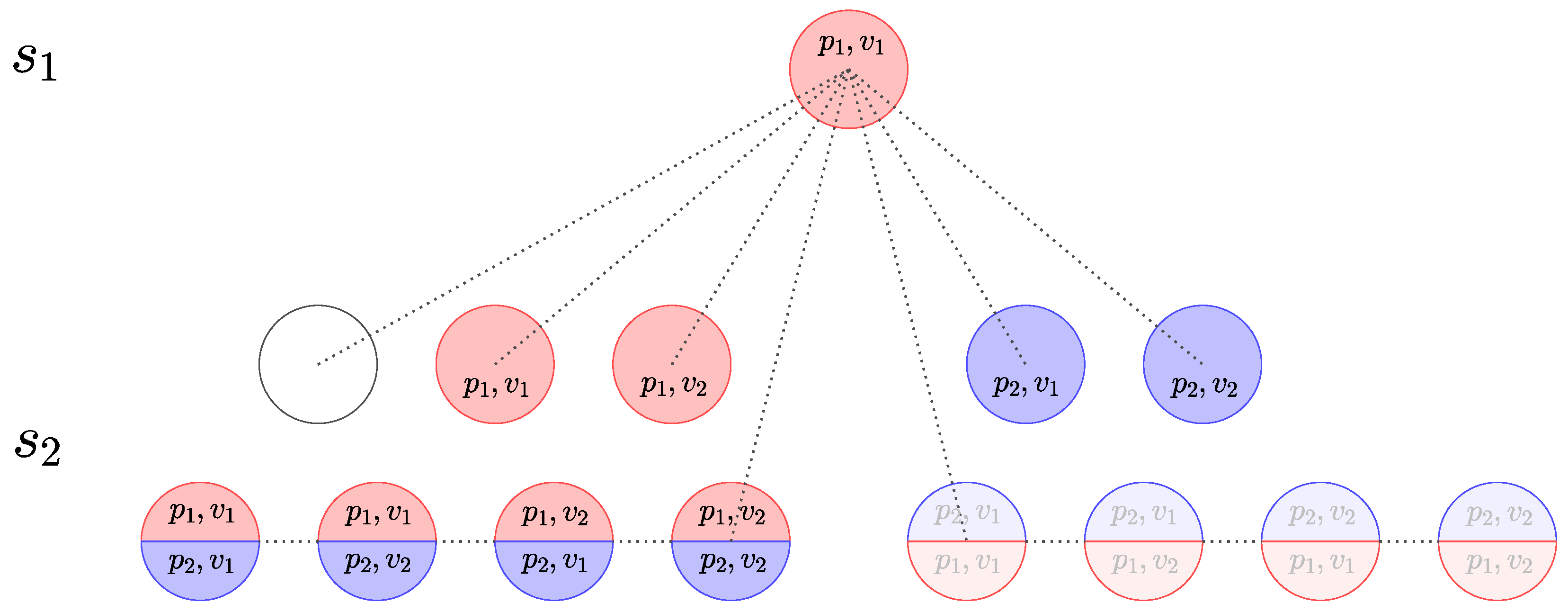
where V is additional information about the speed of the pumps. We assume that is a compact set and that stores the speed control information, , of each pump, , at the operating time step, j. Notice in Figure 2 that with additional speed control options, the number of operation states increases exponentially. Taking into account a range of speed control options, the number of operation states becomes uncountably high.
3. Evaluation of Operation States
For the evaluation of operation states, a surrogate model is used that is trained on real operation data including the information about the total demand of the network, the amount of water stored inside the network, the drinking water inflow and the operating pressure. This model was introduced in [17]. The water system is represented by a system curve of the form
It relates the inflow Q into the network caused by one or more pumps to the delivery head H. The coefficients of the function depend on the current system state, consisting of the drinking water demand, D, and the static height, , which represents the minimum operating pressure of the system.
For the computation of operation data, the system curve is intersected with the current pump curve or, in cases where several pumps run in parallel, a combination of pump curves. The resulting flow rate, Q, and delivery head, H, can then be used to evaluate the key performance indexes, such as power, energy, the change in the drinking water storage container and others. In cases where there is no intersection, the operation is infeasible. Assuming that the operation data is computed every hour, the power, P, to run a pump can be computed by the formula
where is the density of water, g is the gravitational acceleration and is the efficiency of the pump. The power P times the operation time gives the amount of hydraulic energy at that time. The total energy of a schedule is the summation of energy over all operation states. The specific energy, E, is the energy that is used to generate 1 m of drinking water.
For simplification reasons, the notation for the computation of operation data will be skipped. For fixed operating pumps, the energy E is computed according to this section. As will be seen in the next section, the pump curves change with respect to speed and so does the energy. To indicate this influence, the notation is used.
4. Speed Control
In this section, we describe the operation process of speed controlled pumps. Recall from [19] that any pump can be characterized by a characteristic curve,
and an efficiency curve,
Both the delivery head and efficiency are computed from the volume flow rate Q. We assume that both curves are known when the pump is operated at nominal speed.
Let us assume that is the nominal speed (otherwise, your speed can be normalized with respect to the nominal value). When a different speed, , is used, the operation curves scale accordingly. In this paper, the affinity law is used to compute the new dependence of the flow , on the delivery head in terms of the nominal dependence of the flow on the delivery head given by the characteristic curve in Equation (5):
For the computation of efficiency, we use an empirical approach of [20], which scales the nominal efficiency with respect to speed v according to the formula
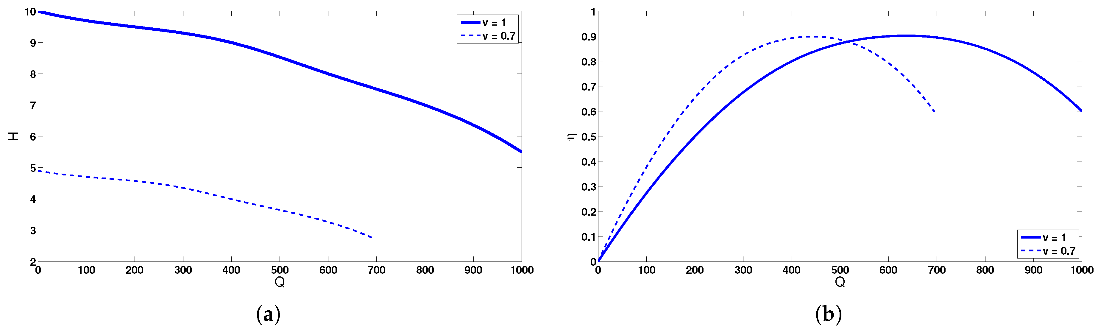
producing , the efficiency of the speed controlled operation. In Figure 3, we show an example where two curves of a pump are scaled with respect to speed . The resulting characteristic curve intersected with the curve of the system yields an appropriate operating state.
5. Optimisation Process
In this section, the operation of a waterworks with variable speed pumps is considered with respect to different constraints. In the first case, we assume that there is a limited number of pump speed options. In the second case, we assume that the pumps can be speed controlled within a fixed speed range, but they can not run in parallel. Finally, we allow both the operation in parallel and with variable speed of pumps.
In the following, we present strategies to generate operation schedules which, in the end, are evaluated as described in Section 3. When more than one key performance indicator is present, solutions to a multicriteria optimization problem are presented. After filtering, only Pareto optimal solutions remain. Filtering is also applied during the solution generation process at each node of the solution tree to save computational time.
5.1. Operation with Finite Number of Speed Control Options
In our previous work [17], we have shown that the number of solutions for the operation problem in Equation (1) grows exponentially with respect to the number of pumps as well as with respect to the number of time periods. Pump speed options enforce additional complexity. They increase the number of operating states at each operating time step . In Section 2, in Figure 1 and Figure 2, it was demonstrated that, after one additional speed control option has been added, the number of operating states increases from 4 to 9 in each branching step. When pumps are assumed, where each pump either runs at one of feasible speeds or is switched off, we have
operating states in each branching step, i.e., in comparison to no speed control, the usage of two additional speed control options squares the number of operating states in each branching step and, thus, the number of solutions is squared for each branching in the so-called solution tree.
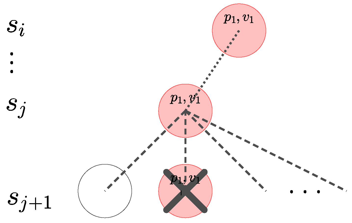
The resulting operation problem stays entirely discrete. The solution tree, which is connected by branching in each node until the final operating time step has been reached, can be traversed in terms of depth first search. Due to the additional complexity, though, it is advisable to limit the number of additional speed control options. In order to improve the computational effort, we recommend using jumps (see Figure 4), i.e., pump combinations are operated until they become infeasible or comparable with an already existing solution in the solution pool. Basically, the problem is equivalent to the operation problem with pumps and, thus, can be treated as in [17].
5.2. Operation on Single Pumps with Variable Speed Control
In this subsection, the speed of a pump is changed continuously with respect to a fixed range, i.e., in Section 4. In addition, the operation at each time step is restricted to a single pump. This is a realistic scenario that has been encountered at the waterworks Barbarossastraße in Kaiserslautern, Germany.
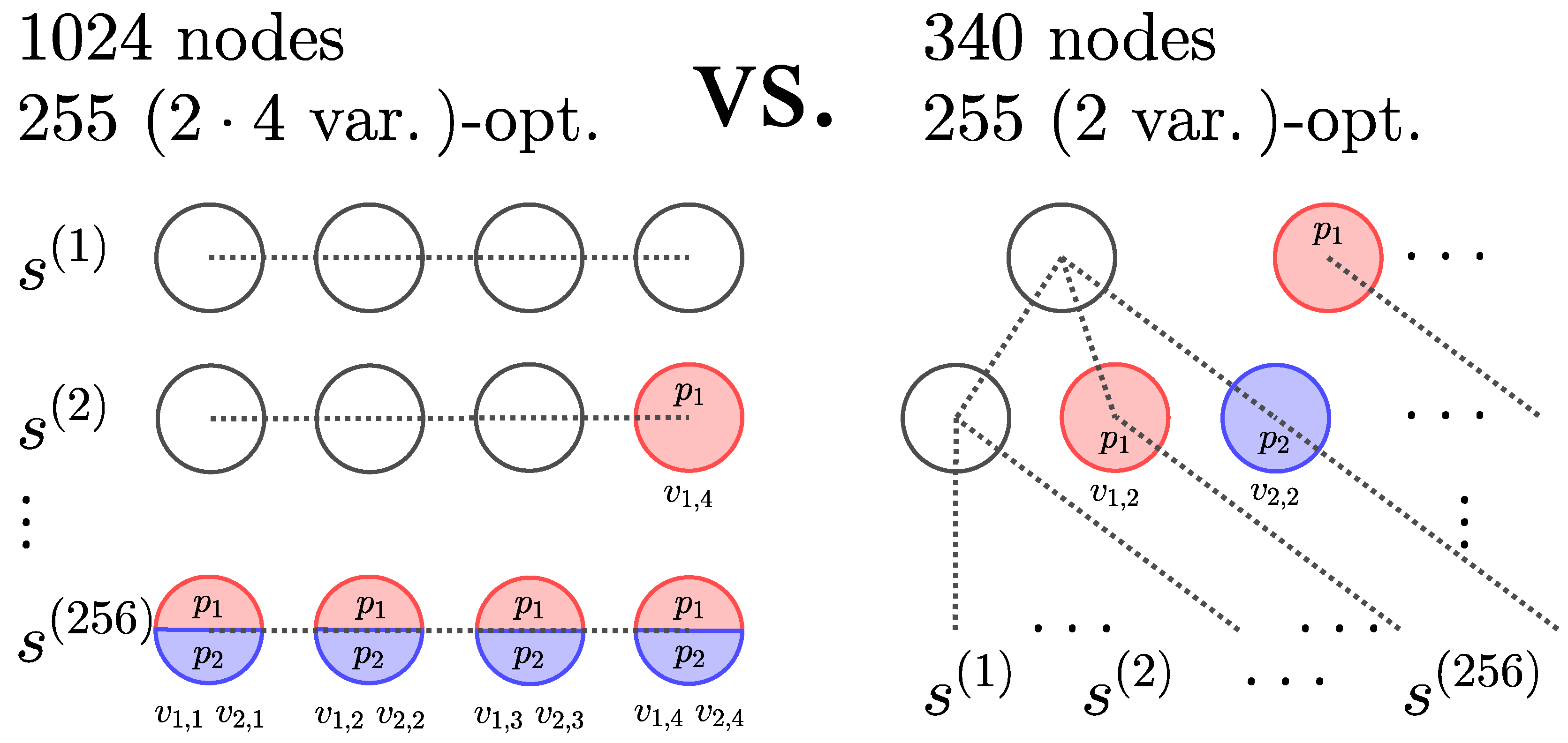
If we wanted to take into account all feasible pump schedules, we would have to consider all possible solutions to the operation problem introduced in Section 2 with no speed control and to optimize each schedule with respect to speed control variables at all points of time, i.e., we would have to optimize each schedule on the left hand side of Figure 5 with single pump operations with respect to m variables. This approach is very inefficient, though. The main reason for this is that, depending on what speed has been chosen at any time step, the flow rate changes according to Section 4 and influences the behavior of the system in all subsequent operating time steps. At worst, each change in speed implies m operation state evaluations. The computational work can not be shared and we cannot cut off partial solutions. It may be that a schedule is infeasible with respect to nominal speed, but it is feasible after pump speed optimization has been applied.
Loosing the ability to share the computational work and to eliminate branches of solutions ahead of time is a big issue. Therefore, we decided to restrict the speed control optimization to single operation time steps. The pump schedule tree, which is illustrated on the right hand side of Figure 5, is traversed analogously to the discrete case, but, at each node, the operation is optimized with respect to speed. After fixing a pump the following optimization problem must be solved:
where is the specific energy used to operate pump at speed v. The operation speed, v, is defined to be feasible if neither the lower bound, , nor the upper bound, , of the water storage container are exceeded by the water level, , during the operation. Notice that concentrating on one single time step makes many objective functions unnecessary. Energy cost deviates very little. There is also no switching allowed within one time step. So, it suffices to increase energy efficiency. The objectives which are more dependent on the schedule are checked during the traversal of the solution tree.
Our solution to the optimization problem in Equation (7) is rather simple. We apply the golden section search from [21]. It is the most effective method that can be applied to general scalar functions. The golden section search expects no conditions on the smoothness of the objective function E. The advantages of using this method are that it is easy to implement, it guarantees that at least a local minimum will be found and, in case of strict unimodality, it guarantees that the optimal solution will be found.
In summary, we suggest that this operation problem is treated similarly to the discrete version from Section 5.1. Branch cutting and jumping from Figure 4 should be applied. The only difference is the additional complexity of finding optimal speed control at each node. After filtering and depth first search traversal, the operation schedules may not be globally optimal, but, they are optimal at each time step. In addition, if necessary, they can still be post-processed.
5.3. Operation on Pumps Running in Parallel with Variable Speed Control
This section considers the operation problem discussed in Section 5.2. However, the restriction of operating on single pumps is dropped, i.e., we allow them to run in parallel [17]. As a consequence, more complexity is added to the optimization of speed control at each time step. The optimization problem in Equation (7) becomes nonlinear multivariate:
In each colored node on the right hand side of Figure 5, this optimization problem needs to be solved. The overall optimization process is treated analogously to Section 5.2.
Golden section search is restricted to univariate optimization. For this reason, we turned to gradient based optimization methods. As indicated by the name, they require the computation of derivatives, in particular, of function E described in Section 3. By relying on data, analytical representation of the specific energy, E, is not available. Hence, numerical differentiation has to be used, which is quite efficient since, typically, the number of pumps is in the tens. We applied the BLEIC algorithm from [22] which uses a nonlinear conjugate gradient method as the underlying optimization algorithm. In comparison to Newton based methods [18], it may require more iterations, but, it forgoes the computation of the Hessian method, which makes each iteration considerably faster.
6. Decision Support Process
In this section, we revisit the navigation described in [17] and extend it, in particular, to address the decision process in the operation of a system where speed control is used. Recall that filtering with respect to the restrictions and modification of an existing solution have been proposed to compare solutions and to convince the user of his final decision interactively. Both can also be done with regard to speed controlled operations. We allow the comparison of speed control options to solutions where none have been applied. The screenshot in Figure 6 illustrates a comparison of two options with respect to two objectives. It shows that the option to operate some pumps at speed 0.9 is more energy efficient. However, the use of speed control requires more switching.
The navigation also helps the user to find speed control options which fit best to the system. After the optimization process with respect to a range of speed control options described in Section 5, the user can select the most preferred schedules. Then, the optimization process can be reset with respect to a finite number of preferred speed control options and the outcome can be compared to the operation of the current system. An example of this process is illustrated in Section 7.
7. Examples
The following examples demonstrate how the suggested optimization process improves the design and operation of both variable and fixed speed pumps. The first example shows the benefit of speed optimization and illustrates the decision process used to find an efficient pump operation schedule. It is shown that the use of the suggested decision process to optimize the operation of variable speed pumps results in an immediate profit for water suppliers who have pumping stations equipped with frequency inverters. The second example demonstrates that the software is also useful for the layout process of a pump, even for systems where pumps are solely operated at a fixed speed. This example uses long-term simulations of pump operation to determine the performance of the current system and to compare changes in performance for different decisions, such as pump adjustment and pump replacement, to the current system.
In both examples, we consider the water supply system which supplies the drinking water demand of the city Worms (Germany). The system can be simplified by the topology depicted in Figure 7. It illustrates a single waterworks operating four pumps to feed the drinking water into the urban network. All four pumps can only be operated at fixed speed. An excess or lack of drinking water is buffered by the storage container. For the definition of the system, please, refer to [17]. Due to unsuitability of old pumps, they were exchanged in 2004 [20]. In order to demonstrate the suggested decision support process in the layout process, we consider the system prior to the pump exchange and refer to this system as the sample system.
7.1. Decision Support for Pump Operation
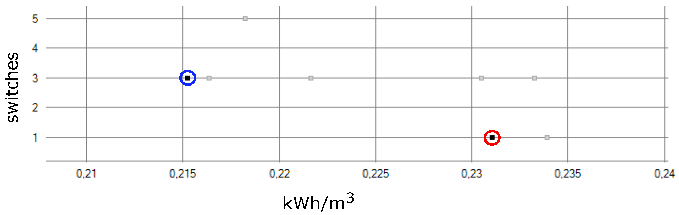
We begin with a decision support process that can be applied to optimize the pump operation process. For this purpose, the consumption data of our sample system was chosen for an arbitrary day and, according to Section 5.2, optimization with respect to pump speed was performed. As a result, the decision support process presents a set of possible pump schedules to the water supplier with respect to their energy efficiencies and the number of switches implied by the schedule (see Figure 8). This navigator view does not just display the best solutions, but also alternatives that deviate within a user-defined tolerance to the objective values of the best solutions. The inferior alternatives can be filtered out (gray dots) to reassure the water supplier in his choice. Clicking on any solution starts an analysis process that presents the operation schedule in detail, i.e., information about the drinking water demand and behavior of the container level during the day, similar to the display in Figure 9.
Let us assume that the water supplier has opted for the most energy efficient solution (blue circle in Figure 8). The pump schedule for this solution can be compared to the identical schedule for pumps operated at a nominal speed, as shown in Figure 9. In general, speed optimized pumps provide less flow and yield a lower container level. The latter means that the pressure in the system is reduced and energy can be saved.
Table 1 confirms that, using speed optimization, water suppliers can operate their pumps more efficiently. In this example, 13% of energy can be saved.
7.2. Decision Support for the Design of the Water Supply System
Beside the optimization of pump operation, the suggested decision support process can be used in the design of the water supply system, as well. More precisely, it can be used for the selection of pumps that better fit the system. The basis of this layout process is a simulation of the sample system with pumps running at nominal speed with respect to sample data for the water demand for one year. This simulation is referred to as the control simulation. Next, similar simulations for the same period of time are performed. The resulting energy expenditures are summarized in Table 2.
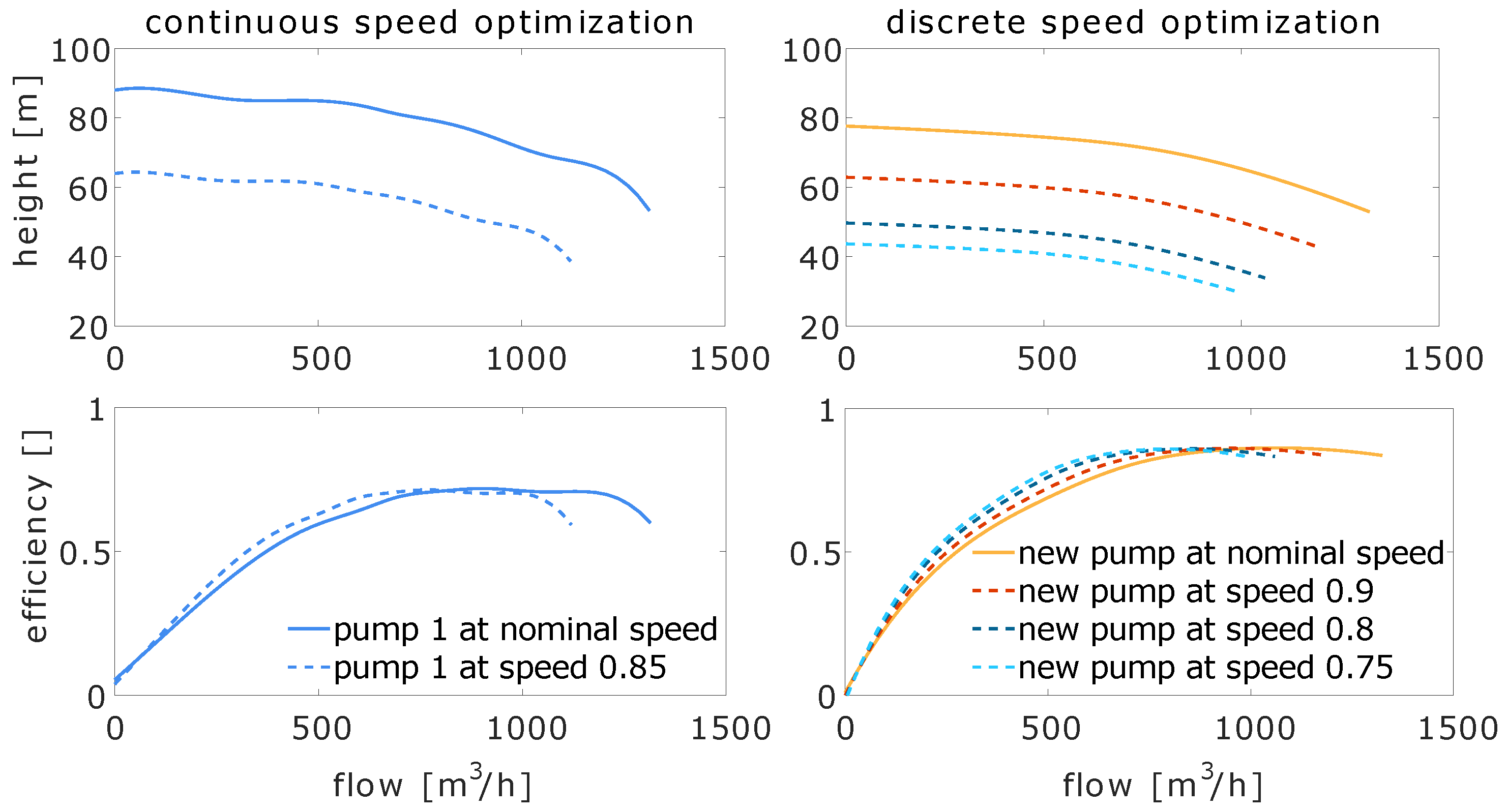
First, the optimization process is used to find out whether the pumps still fit the sample system. For this purpose, system operation is optimized for the sample year with respect to the pump speed according to Section 5.2. Since the goal is the identification of inefficient pumps, for each day of the sample year, the most energy efficient schedule is selected, i.e., other objectives, such as the number of switches, are not taken into consideration. This simulation is referred to as the continuous speed optimization simulation. The resulting statistics, shown in Figure 10, indicate that, during the sample year, the optimization process proposes to use the largest pump (pump 1) most of the time. Furthermore, it optimizes the speed of this pump to an average of 85.25% relative to the nominal speed. Unfortunately, this result can not directly be put into practice, since, in the sample system, pumps can only be operated at the nominal speed. However, we can conclude that pump 1 can not be operated efficiently at the nominal speed. So, as a consequence, either the nominal speed needs to be adjusted or the pump should be replaced. The same statistics in Figure 10 suggest that pump two is used about 10% of the time. Both pump three and pump four are hardly used. Even though this is an indication that two pumps can not be used in the sample system efficiently, the next section focuses on the layout suggestion for pump one.
As mentioned above, the sample system does not allow online speed regulation. However, with little effort, the speed of the pumps can be changed manually. That is, the water supplier can make use of the continuous speed optimization study and adjust the engine speed of pump 1 to 85% of nominal speed, the average optimal speed in Figure 10. However, before changing the system, the effect of this adjustment can be evaluated by optimizing the operation in the sample year with this new fixed speed of pump 1 in the optimization process. The result in Table 2 shows that the new speed of pump 1 has almost 9% of energy savings in comparison to the operation at nominal speed.
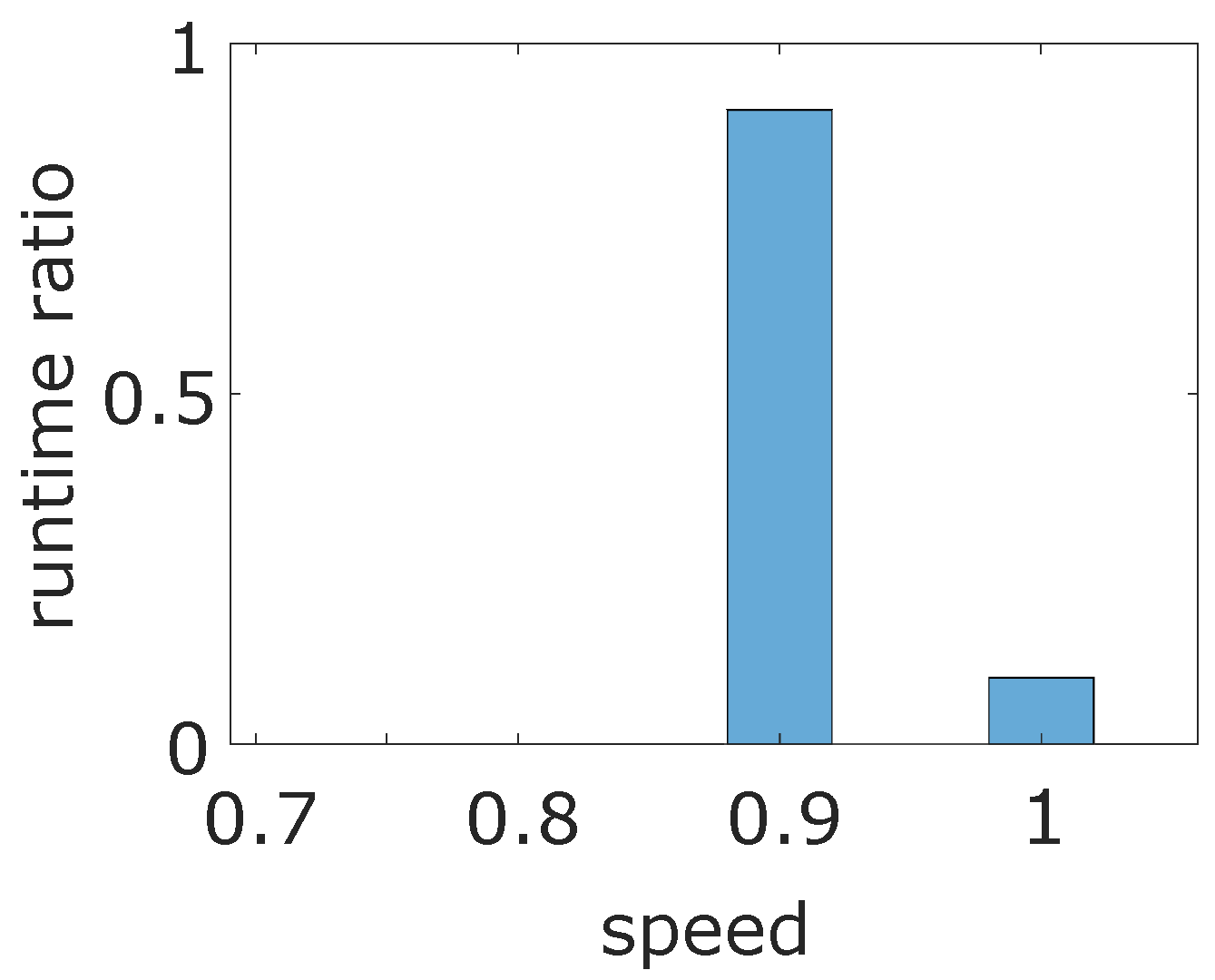
Finally, the optimization process can accompany the water supplier through the process of choosing a new pump. Suppose that the water supplier has decided to replace pump 1 in the sample system. Using the discrete speed optimization discussed in Section 5.1, a new pump candidate is tested for the speed values relative to the nominal speed to determine the speed that the new pump should be adjusted to in the system (see Figure 11). Figure 12 displays the discrete optimization result: At 90% of operation time, the new pump is operated at 90% relative to the nominal speed, whereas at 10% of operation time, the pump runs at the nominal speed. Replacing pump 1 in the sample system by this pump, adjusted to 90% relative to the nominal speed, the optimization process predicts that the operator will save up to 18% of energy compared to the nominal speed scenario (see Table 2).
As summarized in Table 2, the water supplier can compare the effects of different courses of action with respect to energy expenditure. Based on the simulations of different scenarios, he can decide to keep the system unchanged, to adjust the speed of pump 1, which would save about 9% of energy, or to spend money on a new pump with a predicted 18% in yearly energy savings.
Overall, this example has demonstrated an application of the proposed optimization process and the decision support process to identify inefficient pumps in a water supply system. Furthermore, we have shown how to use the proposed optimization process in the evaluation and the layout process of existing systems.
8. Conclusions
In this paper, we have presented an optimization process and an extended decision support process for the design and operation of water supply systems, with an emphasis on the use of variable speed pumps. It has been applied to a model of the water supply system at Worms, Germany. Different scenarios have been compared using an optimization process which predicted yearly energy savings of up to 18%. Currently, the suggested changes cannot be applied at Worms. However, the extensive comparison of the surrogate hydraulic model with real data was performed in [23] showing that the model deviates, on average, by with a standard deviation of . This deviation is rather small in comparison to 18%, i.e., an energy saving of the same amount is very realistic.
The hydraulic model used in this paper is rather simple, but it can be used to model many similar water supply companies in Germany. The main requirement for the introduced method to work well is that the system can be modeled in such a way that the computation of operation points is not costly. This has been the case in this paper due to the use of an approximating system curve model. One weakness of the branch and bound method is the exponential growth of time complexity. However, in Section 5, suggestions have been made to help to keep time complexity at bay.
The next step is to develop new methods using operation data to approximate more complex systems consisting of several water storage containers and drinking water consumption areas. We plan to cooperate with more water supply companies and to implement the suggested decision support process into their systems.
Author Contributions
D.N. designed the concept of this paper, developed the model code and wrote the paper. H.K. performed the simulations. C.G. and A.K. were responsible for the hydraulic modelling and assessment of the water utilities. M.B. and H.R. contributed a critical revision of the paper.
Acknowledgments
This work is part of the project Opt which is funded by the Federal Ministry of Education and Research of Germany.
Conflicts of Interest
The authors declare no conflict of interest.
References
- Mala-Jetmarova, H.; Sultanova, N.; Savic, D. Lost in Optimisation of Water Distribution Systems? A Literature Review of System Design. Water 2018, 10, 307. [Google Scholar] [CrossRef]
- Branchenbild der Deutschen Wasserwirtschaft; wvgw Wirtschafts- und Verlagsgesellschaft Gas und Wasser: Bonn, Germany, 2015.
- Energieeinsparung; Grundfoss Pressetext: Erkrath, Germany, 2017.
- Coelho, B.; Andrade-Campos, A. Efficiency achievement in water supply systems—A review. Renew. Sustain. Energy Rev. 2014, 30, 59–84. [Google Scholar] [CrossRef]
- Kiselychnyk, O.; Bodson, M.; Werner, H. Overview of Energy Efficient Control Solutions for Water Supply Systems; Transactions of Kremenchuk State Polytechnic University: Kremenchuk, Ukraine, 2009; Volume 3, pp. 40–45. [Google Scholar]
- Ormsbee, L.; Lansey, K. Optimal Control of Water Supply Pumping Systems. J. Water Resour. Plan. Manag. 1994, 120, 237–252. [Google Scholar] [CrossRef]
- Westphal, K.S.; Vogel, R.M.; Kirschen, P.; Chapra, S.C. Decision Support System for Adaptive Water Supply Management. J. Water Resour. Plan. Manag. 2003, 129, 165–177. [Google Scholar] [CrossRef]
- Georgescu, S.-C.; Georgescu, A.-M. Application of HBMOA to Pumping Stations Scheduling for a Water Distribution Network with Multiple Tanks. Procedia Eng. 2014, 70, 715–723. [Google Scholar] [CrossRef]
- Behandish, M.; Wu, Z.Y. Concurrent Pump Scheduling and Storage Level Optimization Using Meta-models and Evolutionary Algorithms. Procedia Eng. 2014, 70, 103–112. [Google Scholar] [CrossRef]
- Scarpa, F.; Lobba, A.; Becciu, G. Expeditious Pump Rescheduling in Multisource Water Distribution Networks. Procedia Eng. 2015, 119, 1078–1087. [Google Scholar] [CrossRef]
- Blinco, L.J.; Simpson, A.R.; Lambert, M.F.; Auricht, C.A.; Hurr, N.E.; Tiggemann, S.M.; Marchi, A. Genetic Algorithm Optimization of Operational Costs and Greenhouse Gas Emissions for Water Distribution Systems. Procedia Eng. 2014, 899, 509–516. [Google Scholar] [CrossRef]
- Brentan, B.M.; Luvizotto, E., Jr.; Montalvo, I.; Izquierdo, J.; Pérez-García, R. Near Real Time Pump Optimization and Pressure Management. Procedia Eng. 2017, 186, 666–675. [Google Scholar] [CrossRef]
- Menke, R.; Abraham, E.; Parpas, P.; Stoianova, I. Approximation of System Components for Pump Scheduling Optimisation. Procedia Eng. 2015, 119, 1059–1068. [Google Scholar] [CrossRef]
- Miettinen, K. Nonlinear Multiobjective Optimization; International Series in Operations Research and Management Science; Springer: New York, NY, USA, 1999. [Google Scholar]
- Ehrgott, M. Multicriteria Optimization; Springer: Berlin, Germany, 2005. [Google Scholar]
- Land, A.H.; Doig, A.G. An automatic method for solving discrete programming problems. Econometrica 1960, 28, 497–520. [Google Scholar] [CrossRef]
- Nowak, D.; Bortz, M.; Roclawski, H. Decision Support for the Design and Operation of Water Supply Systems. Procedia Eng. 2015, 119, 442–449. [Google Scholar] [CrossRef]
- Ruszczynski, A. Nonlinear Optimization, 1st ed.; Princeton University Press: Princeton, NJ, USA, 2006. [Google Scholar]
- Hellmann, D.-H. KSB-Kreiselpumpen-Lexikon, 4th ed.; KSB: Frankenthal, Germany, 2009. [Google Scholar]
- Pfleiderer, C. Die Kreiselpumpen für Flüssigkeiten und Gase, 4th ed.; Springer: Berlin, Germany, 1955. [Google Scholar]
- Jarre, F.; Stoer, J. Optimierung; Springer: Berlin, Germany, 2004. [Google Scholar]
- Box and Linearly Constrained Optimization. Available online: http://www.alglib.net/optimization/boundandlinearlyconstrained.php (accessed on 4 June 2018).
- Krieg, H.; Nowak, D.; Bortz, M.; Knapp, A.; Geil, C.; Roclawski, H.; Böhle, M. Decision support for planning and operation of drinking-water supply systems [Entscheidungsunterstützung für planung und Betrieb von Trinkwasserversorgungsanlagen]. GWF Wasser Abwasser 2016, 157, 746–756. [Google Scholar]
Figure 1.
Branching for the pump operation in the second time step after pump has been operated in the first time step. The colors red, blue and no color represent pumps and and no pump.
Figure 1.
Branching for the pump operation in the second time step after pump has been operated in the first time step. The colors red, blue and no color represent pumps and and no pump.

Figure 2.
Branching for the pump operation with two speed control options and . The colors red, blue and no color represent pumps and and no pump. Faded nodes represent duplicates.
Figure 2.
Branching for the pump operation with two speed control options and . The colors red, blue and no color represent pumps and and no pump. Faded nodes represent duplicates.

Figure 3.
The characteristic curve in (a) and the efficiency curve in (b) are both scaled down from speed to speed .
Figure 3.
The characteristic curve in (a) and the efficiency curve in (b) are both scaled down from speed to speed .

Figure 4.
Solution tree traversal with jumps: After choosing to operate pump at speed at operating time step , the operation is continued until the operation is no longer feasible at step , i.e., the storage container overflows, or the intermediate solution can be compared to previously computed solutions.

Figure 5.
Variable speed optimization comparison for the pump operation . On the left hand side, each schedule is optimized with respect to at most variables for speed . On the right hand side, optimization is performed at each colored node with respect to, at most, variables. In both cases, the same number of optimization problems has to be solved (255), but, the problems to solve are simpler on the right hand side (two instead of eight variables). Red, blue and no color represent pumps and and no pump, respectively.

Figure 6.
Comparison to speed control. Red solutions operate pumps with a nominal speed. Green solutions operate pumps at speed of 0.9.
Figure 6.
Comparison to speed control. Red solutions operate pumps with a nominal speed. Green solutions operate pumps at speed of 0.9.

Figure 7.
Water supply system with a single water storage container and four pumps.

Figure 8.
Decision support system for pump operation: The software presents the best solutions concerning the specific energy (blue circle) and number of switches (red circle). Inferior solutions are filtered out.
Figure 8.
Decision support system for pump operation: The software presents the best solutions concerning the specific energy (blue circle) and number of switches (red circle). Inferior solutions are filtered out.

Figure 9.
Pump schedule with pumps running at a nominal speed (upper panel) compared to the pump schedule resulting from speed optimization (second panel). In the lower panel, the optimized speeds of the pumps in the second panel are shown.
Figure 9.
Pump schedule with pumps running at a nominal speed (upper panel) compared to the pump schedule resulting from speed optimization (second panel). In the lower panel, the optimized speeds of the pumps in the second panel are shown.

Figure 10.
Pump operation statistics for the year 2012.

Figure 11.
Characteristic curves and efficiency curves of the pumps used in the optimization runs.

Figure 12.
Discrete speed optimization result for the sample water demand of one year.


Table 1.
Energy savings when operating speed optimized pumps.
| Operation at Nominal Speed | Operation at Optimized Speed | |
|---|---|---|
| specific energy ( | 0.24855 | 0.21525 (86.6%) |
| total energy (kWh) | 4.471 | 3.872 (86.6%) |
Table 2.
Energy savings for optimized speed control.
| Control Simulation | Cont. Speed Optimization | Pump One Fixed at Speed 0.85 | Discrete Speed Optimization for a New Pump | |
|---|---|---|---|---|
| specific energy ( | 0.24453 | 0.22325 (91.3%) | 0.22393 (91.6%) | 0.19963 (81.6%) |
| total energy (kWh) | 1.659.387 | 1.513.923 (91.2%) | 1.518.704 (91.5%) | 1.354.214 (81.6%) |
© 2018 by the authors. Licensee MDPI, Basel, Switzerland. This article is an open access article distributed under the terms and conditions of the Creative Commons Attribution (CC BY) license (http://creativecommons.org/licenses/by/4.0/).
Share and Cite
MDPI and ACS Style
Nowak, D.; Krieg, H.; Bortz, M.; Geil, C.; Knapp, A.; Roclawski, H.; Böhle, M. Decision Support for the Design and Operation of Variable Speed Pumps in Water Supply Systems. Water 2018, 10, 734. https://doi.org/10.3390/w10060734
AMA Style
Nowak D, Krieg H, Bortz M, Geil C, Knapp A, Roclawski H, Böhle M. Decision Support for the Design and Operation of Variable Speed Pumps in Water Supply Systems. Water. 2018; 10(6):734. https://doi.org/10.3390/w10060734
Chicago/Turabian StyleNowak, Dimitri, Helene Krieg, Michael Bortz, Christian Geil, Axel Knapp, Harald Roclawski, and Martin Böhle. 2018. "Decision Support for the Design and Operation of Variable Speed Pumps in Water Supply Systems" Water 10, no. 6: 734. https://doi.org/10.3390/w10060734
Note that from the first issue of 2016, this journal uses article numbers instead of page numbers. See further details here.