Validation of a Computational Fluid Dynamics Model for a Novel Residence Time Distribution Analysis in Mixing at Cross-Junctions

Abstract

In Water Distribution Networks, the chlorine control is feasible with the use of water quality simulation codes. EPANET is a broad domain software and several commercial computer software packages base their models on its methodology. However, EPANET assumes that the solute mixing at cross-junctions is “complete and instantaneous”. Several authors have questioned this model. In this paper, experimental tests are developed while using Copper Sulphate as tracer at different operating conditions, like those of real water distribution networks, in order to obtain the Residence Time Distribution and its behavior in the mixing as a novel analysis for the cross-junctions. Validation tests are developed in Computational Fluid Dynamics, following the k-ε turbulence model. It is verified that the mixing phenomenon is dominated by convection, analyzing variation of Turbulent Schmidt Number vs. experimental tests. Having more accurate mixing models will improve the water quality simulations to have an appropriate control for chlorine and possible contaminants in water distribution networks.

1. Introduction

In recent years, useful life of a several number of Water Distribution Networks (WDN) has been exceeded, so that there are certain points or sectors that do not reach enough disinfectant. This problem could produce the formation of biofilm on pipe walls [1,2], promoting bacterial growth and its transport through water. On the other hand, the system's own useful life, the intermittency in the supply, the leaks level, and the demands behaviour cause a great variety of residence times of the drinking water and variations of reaction of the disinfectant in the network [3,4].

Chlorine disinfection is one of the principal factors in drinking water treatment processes. This chemical agent is used mainly to ensure the destruction of pathogen organisms that could be present in water and that are coming from the sources of supply. The disinfection prevents gastrointestinal diseases due to the consumption of contaminated water. However, it is also true that chemical disinfection has caused unwanted risks due to by-products that are generated in the reactions with contaminants present in water, such as trihalomethanes (THM), among others [1,2,5,6,7,8,9].

Finding solutions to the problem of inadequate use of chlorine is an issue that involves various aspects. When WDN presents a high degree of reaction due to pipe conditions and residence times, concentrations in some areas decrease rapidly [2,3,7]. Due to this, the absence of the necessary amount of disinfectant induces the possible consumption of water that is contaminated by users. A commonly used solution is the increased chlorine concentration from the sources. However, demand nodes near the sources distribute water with the high chlorine contents and due to factors, such as residence times, the formation of harmful by-products increases, which in the same way affects the consumer population [9,10].

Location of strategic points to control the problem of some solute distribution can be reached through the applications, in which it is necessary to improve the incomplete mixing model. Diverse authors [11,12,13,14] have developed models based on heuristic technics that use the results of water quality analysis to determine the best location of booster chlorination stations to optimize their usage. Other authors [15,16,17,18,19,20] developed researches that determine the strategic zones for the sensors location to detect pollutants, with the aim of finding accidental or intentional action of harmful agents and with the idea that the consumer has the risk of consuming contaminated water. Both kinds of applications predict the best zones for the water quality control devices; however, they are dependent on the way, in which EPANET (is a computer program that performs extended period simulation of hydraulic and water quality behavior within pressurized pipe networks [21]. The name comes from the U.S. Environmental Protection Agency and Networks) simulates the distribution of a solution through the network; the predictions are not accurate as many cross-junctions are presented in the networks that are studied.

An incomplete mixing analysis is presented in experimental tests that use injection pulses of copper sulphate (CuSO₄) as a tracer. Residence Time Distribution (RTD) curves are good features and a novel proposal on mixing cross-junctions, in order to calibrate simulation processes, with the help of stimulus-response techniques [22,23,24]. There were generated turbulent regime scenarios in Reynolds numbers from 43,343 to 155,793. Therefore, different operating conditions that are close to real WDN were performed. To analyse the tracer distribution in the outlets of the cross-junction, the curves of the pulses are registered, visualizing by RTD curves the approximation of the Computational Fluid Dynamics (CFD) simulations. According to the cross-junction mixing models that are reviewed in the literature, this is the first time that the hydraulic pipe flow has been simulated with success using RTD analysis, which was addressed by solving the RANS equations with the k-epsilon turbulence model coupled to the diffusion-convection equation.

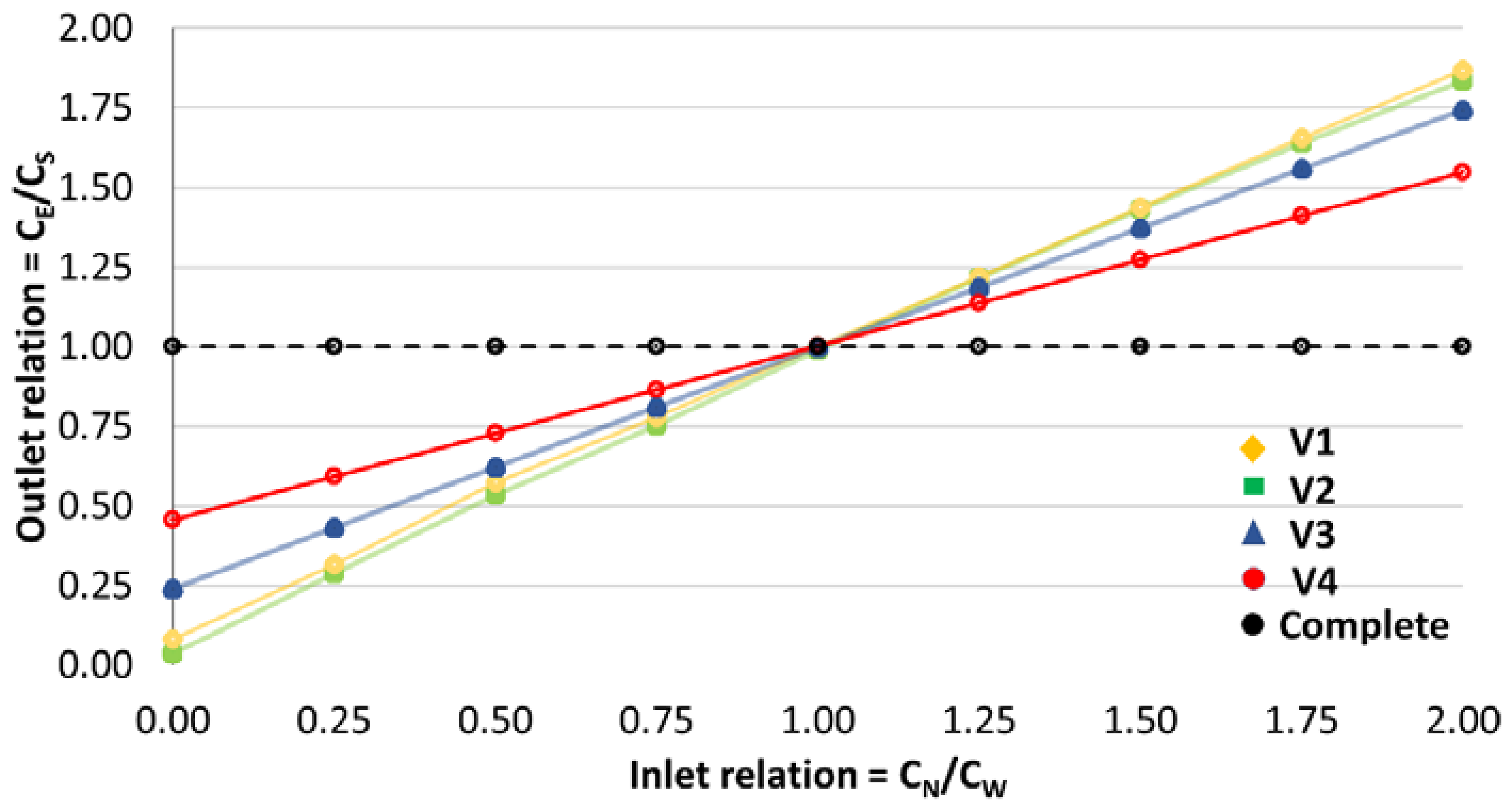
Complete Mixing Model

In EPANET and in most hydraulic simulation programs, it is assumed that the solute mixing is complete and instantaneous [21]. Therefore, the concentration of the substance (for example: residual chlorine) that leaves the cross-junction, will be the weighted average of the solute concentrations of the arriving pipes. For a given node k, the concentration leaving the node is obtained by Equation (1).

$$C_i=\frac{{{\displaystyle \sum }}_{j\in I_k}{Q}_j{C}_j+Q_{k,ext}{C}_{k,ext}}{{{\displaystyle \sum }}_{j\in I_k}{Q}_j+Q_{k,ext}}$$

(1)

where: i, link with flow leaving node k; I_k, set of links with flow into k; L_j, length of link; Q_j, flow (volume/time) in link j; Q_k,ext, external source flow entering the network at node k; and, C_k, _ext, concentration of the external source flow entering at node k.

Several authors [25,26,27,28,29,30,31,32,33,34,35,36] have numerically and experimentally demonstrated that the mixing in these unions is far from being “complete and instantaneous”. Most of these researches were based on physical experiments and simulations through Computational Fluid Dynamics (CFD) using tracers for the concentration distribution analysis. Some researchers [26,27,28,31,32,33,34,35,36] implement experimental scale models of a cross-junction and tee junctions with different pipe diameters, which are driven by elevated tanks where tracer is injected into one of them. Once the mix of the flows was made, mixing coefficients were formulated based on their experimental measurements. Some others based their approaches on CFD simulations directly, even for small geometric configurations [25,29,30]. The most commonly used tracers were salts, such as NaCl. Other authors considered colored dyes and high speed photography too [34,35]. Conducting a study directly with chlorine as a solute turns out to be somewhat complicated, although Mompremier [33] used in-line chlorine loggers/dosers to analyze the mixing at different conditions.

The developed studies carried out to date allow for the derivation of mathematical functions for the computation of the incomplete mixing, even two codes have been formulated to be implemented as toolkits for EPANET (one of them, called AZRED II and developed by [36]). However, these applications have not been disseminated globally yet, because most of them were performed by scaled experimental devices reaching low velocities and turbulent flows that were close to 4000. In some cases, they are still subject to specific calibrations of each network and there is a lack of experimental sufficiency in real networks of high interconnection.

The lack of precision in water quality simulations can lead to erroneous projects of monitoring systems of the location of re-chlorination systems necessary for the control of disinfection [28]. The accuracy in these models is also necessary to simulate the spatial-temporal dispersion of chemical and microbial agents during accidental or intentional contamination events.

This paper presents a validation of the phenomenon of mixing in cross-junctions by means of CFD, in which the distribution of the disinfectant is not considered as homogenous mixing. The presented scenarios were performed at velocity and pressure conditions that were similar to those real WDN thanks to the impulsion and conduction equipment used. This avoids making measurement adjusts or extrapolations, that makes it different from many other jobs working at lower turbulence flows. The model is validated by a novel analysis of RTD curves for mixing cross-junction, resulting from the execution of tests of different velocity conditions and its corresponding measurement of copper sulfate injection response. The correct model meshing degree is verified for the study of the phenomenon in the CFD model.

2. Materials and Methods

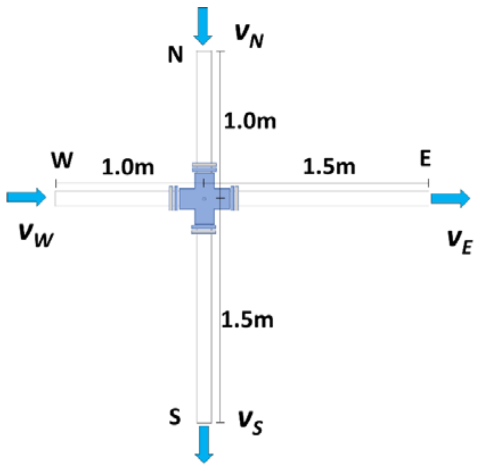
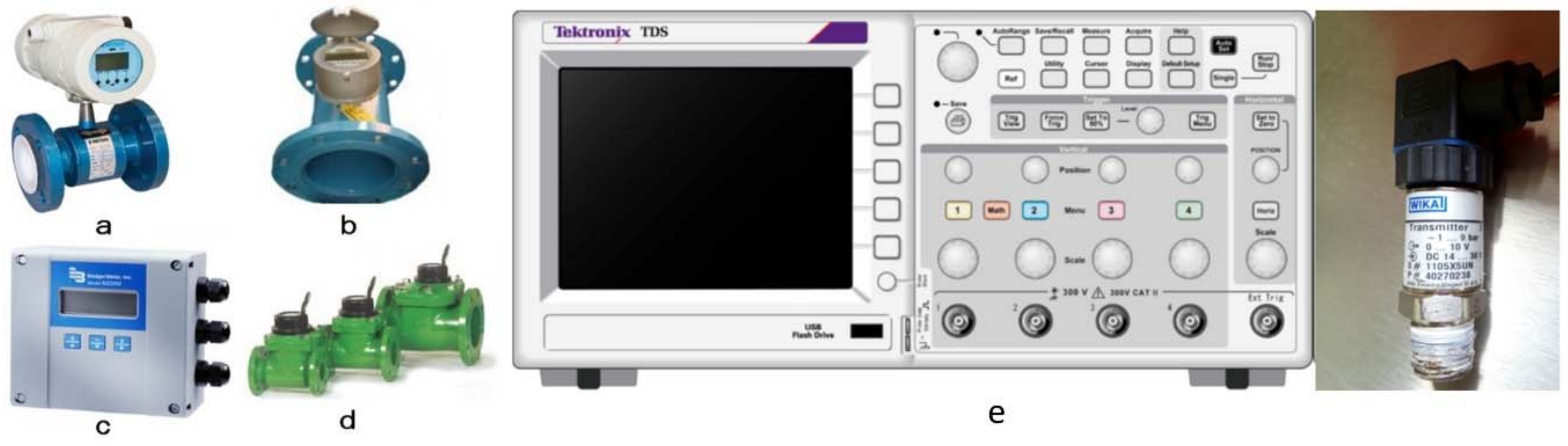
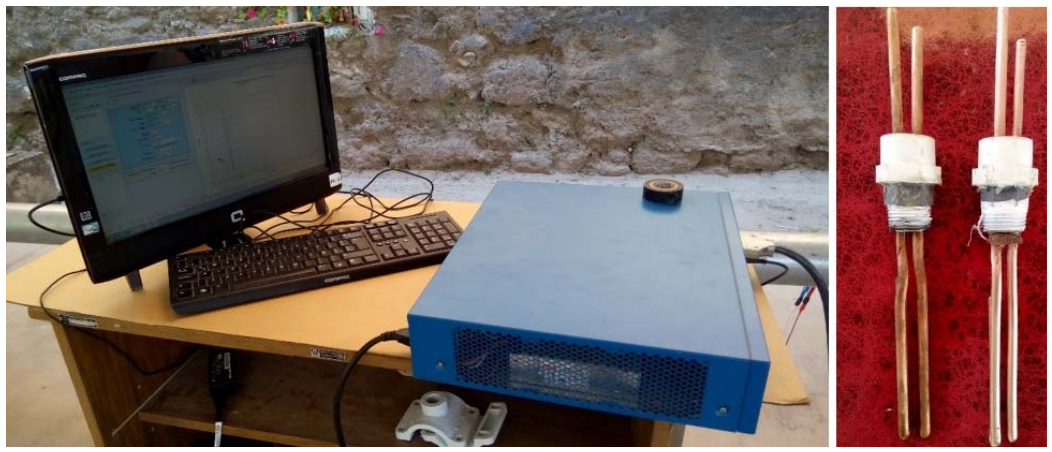
2.1. Experimental Model

The cross-junction used for the mixing analysis is situated on an experimental network of the “Universidad de Guanajuato”; the pipe material is galvanized iron of four inches in diameter (Figure 1). The flows are conducted by a 15HP hydraulic pump, which reaches 30 L per second at pressures of 1.78 bar for the pipes on the cross-junction. Open valves are available at each border for flow velocity control for inlets and outlets. They are located at 2 and 7.5 m upstream water from the cross-junction. It is done to reduce turbulence generated by the obstruction of the valve, and so that the flow could be uniformized along the pipeline.

Operating conditions that are close to WDN can be approximated by the physical characteristics of the experimental network. All of the mixing tests were developed contemplating two inlets and two outlets flow. The boundary distances (shown in Figure 1), that were established for the numerical model, are the location points of the pressure measuring devices. The north inlet (N) corresponds to the upper boundary. The West inlet (W) is the left boundary, and in the same way for the outlets boundaries on the East (E) and South (S) (Figure 1). In addition, the numerical model is performed with the objective of maintaining the flow direction with a sense from left to right and from top to bottom.

North and West inlets flows are measured with the support of two flow meters, of them being of electromagnetic type, DOROT brand, model MC608-A (Figure 2a). The second one is a propeller meter, of the company Hidrónica^®, model MP-0400 (Figure 2b), both with datalogger capabilities. For measures at the outlets, the outflowing water is conducted up to four flowmeters, two for each outlet. For the East outlet, the flowmeters are of electromagnetic type, of Badger Meter Inc. brand, model M2000 (Figure 2c). For the South outlet, the water is conducted to two propeller volumetric flow meters (Figure 2d).

A digital storage oscilloscope with four measuring channels, a Tektronix^® brand model TDS-2004C (Figure 2e) was available to the pressure registration on the four boundaries of the cross-junction. In this case, the oscilloscope visually represents the electrical signals that are captured by pressure transducers. These transducers are of WIKA^® brand model S-10, comprise a measuring range of 0–10 V of electrical signal intensity corresponding to the range −1 to 9 bar of pressure.

The tracer that was used for the tests is copper sulphate pentahydrate (CuSO₄·5H₂O) of fine grade, Fermont^® brand. The 0.25 mol/L solutions are prepared, which return an effective response to the concentration measurement. The tracer injection is done by pumping, with a monophasic equipment, Siemens brand, 1HP power and rotor speed of 3515–3535 rpm. The tracer is stored in a volumetric test tube of four liters size, and then, in each test, the tracer is pumped 150 mL approximately. The injection point is located at 3.50 m before the cross-junction (Figure 3). The pump equipment allows for overcoming the pressures of water flow in the network and the controlled intrusion of tracer that is injected through the opening and closing ball valve of a 0.5 inch.

A potentiostat-galvanostat, brand BIOLOGIC, model SP-150 was used to apply an electric potential, with which copper adhesion will occur on the electrodes (Figure 4). This equipment has software that allows for current intensity registration at fixed time intervals. The electrodes were placed at the outlet boundaries of the pipes, close to the pressure transducers. The electrodes must be made of a metal with suitable properties for electrical conduction. They were developed with the characteristics that are shown in the

Table 1. Characteristics of the electrodes.

Material	Solid Copper
Electrode diameter	4.4 mm
Length of electrodes	9.5 cm (covers more than 90% of the pipe diameter)
Electrodes separation	4.6 mm
Insulation material	resin

.

The velocity alternatives for the case of two inlets and two outlets are described in Figure 5. To simulate equal velocities is difficult because of working with high magnitudes of velocity and pressure. Therefore, the scenarios were approximated as much as possible to cover the four-velocity combinations in Figure 5. It has been determined that the flow velocities are closer when the variation between both of the inlets or outlets boundaries are by a percentage with a relative difference is less than 25%, otherwise, for the variations that are presented with a relative difference of 25% or greater, it is considered that the velocities are different. The objective is to cover trials that involve the different mixing conditions, likely in a cross joint. The alternatives are classified in these four groups, according to their velocities.

Table 2. Contents values of the four scenarios V1 to V4 proposed.

Front		V1				V2				V3				V4
		V (m/s)	P (bar)	Re	Q (l/s)	V (m/s)	P (bar)	Re	Q (l/s)	V (m/s)	P (bar)	Re	Q (l/s)	V (m/s)	P (bar)	Re	Q (l/s)
Inlets	N	1.112	1.88	112,928	9.01	1.116	1.60	113,396	9.05	0.808	1.57	82,123	6.55	0.672	1.96	68,295	5.45
	W	1.059	1.88	107,625	8.59	1.269	1.60	128,971	10.29	1.533	1.56	155,793	12.43	0.989	1.96	100,503	8.02
Outlets	E	1.005	1.88	102,067	8.14	1.062	1.56	107,899	8.61	1.039	1.56	105,654	8.43	1.246	1.96	126,624	10.10
	S	1.167	1.88	118,547	9.46	1.324	1.56	134,468	10.73	1.302	1.56	132,273	10.55	0.427	1.96	43,343	3.46

contains contents values of the four scenarios V1 to V4 proposed.

2.2. Formulation of Numerical Simulation

2.2.1. Turbulent Flow

The numerical simulations for the dynamic flow are based on the mass conservation Equation (2) and the Reynolds Averaged Navier-Stokes (RANS). These last equations consider the turbulent flow applying Reynolds decomposition by its average over a small-time increment; the flow quantities are decomposed in a temporal mean and a fluctuating component [37]. The decomposition results in the RANS Equation (3) [38,39].

$$\nabla ·\left(\rho u\right)=0$$

(2)

$$\rho \left(u·\nabla \right)u=-\nabla P+\nabla ·\left(\left(\mu +{\mu }_T\right)\left(\nabla ·u+{\left(\nabla ·u\right)}^T\right)\right)$$

(3)

where u is the mean-averaged velocity vector, P is the pressure, µ is the dynamic viscosity, and ρ is the fluid density.

The fluctuating component introduces a closure problem [37], which could be solved by diverse type of models: Eddy Viscosity or First-Order and Second-Moment Closure (SMC). The standard k-ε model is one of SMC that works with high Reynolds number turbulence valid only for fully turbulent free shear flows that cannot be integrated all the way to the wall [40]. Modeling flows close to solid walls requires integration of the two equations over a fine grid to correctly capture the turbulent quantities inside the boundary layer [40,41]. Then, the so-called Reynolds stresses can be stated in terms of a turbulent viscosity µ_T, according to the standard k-ε turbulence model; Equations (4) to (6).

$${\mu }_T=\rho C_{\mu }\frac{k^2}{\epsilon }$$

(4)

$$\rho \left(u\nabla \right)k=\nabla ·\left(\left(\mu +\frac{{\mu }_T}{{\sigma }_k}\right)\nabla k\right)+P_k-\rho \epsilon$$

(5)

$$\rho u·\nabla \epsilon =\nabla ·\left(\left(\mu +\frac{{\mu }_T}{{\sigma }_{\epsilon }}\right)\nabla \epsilon \right)+C_{e1}\frac{\epsilon }{\kappa }{P}_k-C_{e2}\rho \frac{{\epsilon }^2}{k}$$

(6)

where k is the turbulent kinetic energy, ε is the turbulent energy dissipation rate, P_k is the energy production term ($P_k={\mu }_T[\nabla u:(\nabla u+{(\nabla u)}^T]$), and C_µ (0.09), C_e1 (1.44), C_e2 (1.92), σ_k (1), and σ_ε (1.3) are dimensionless constant values that are obtained by data fitting over a wide range of turbulent flows [38]. K. Hanjalik [41] used the k-ε model over other types of turbulence models for simulation in pressure pipes with high Reynolds numbers, with the same empirical constants. Furthermore, RANS k-ε models have proposed good results also in mixing and concentration analysis, when these models have been validated with measurements, as in [42,43].

2.2.2. Boundary Conditions

Due to the high values of the Reynolds number that were reached in the scenarios, velocities in regions near the walls model decrease rapidly. The fluid velocity becomes dependent on these boundaries. The wall functions used are based on a universal distribution of velocities depending on the proximity of the wall, Equation (7).

$$u^{+}=\frac{1}{\kappa }\ln \left(E{y}^{+}\right)$$

(7)

where u⁺ is the normalized velocity component in the logarithmic layer of the wall, κ is the Von Karman constant (0.4187), E is a constant that depends on the roughness of the wall, and y⁺ is the dimensionless distance from the wall.

The input parameters that are assigned to the CFD analysis (shown in Table 2) were established them in the following way, at the same distance like in the experimental model:

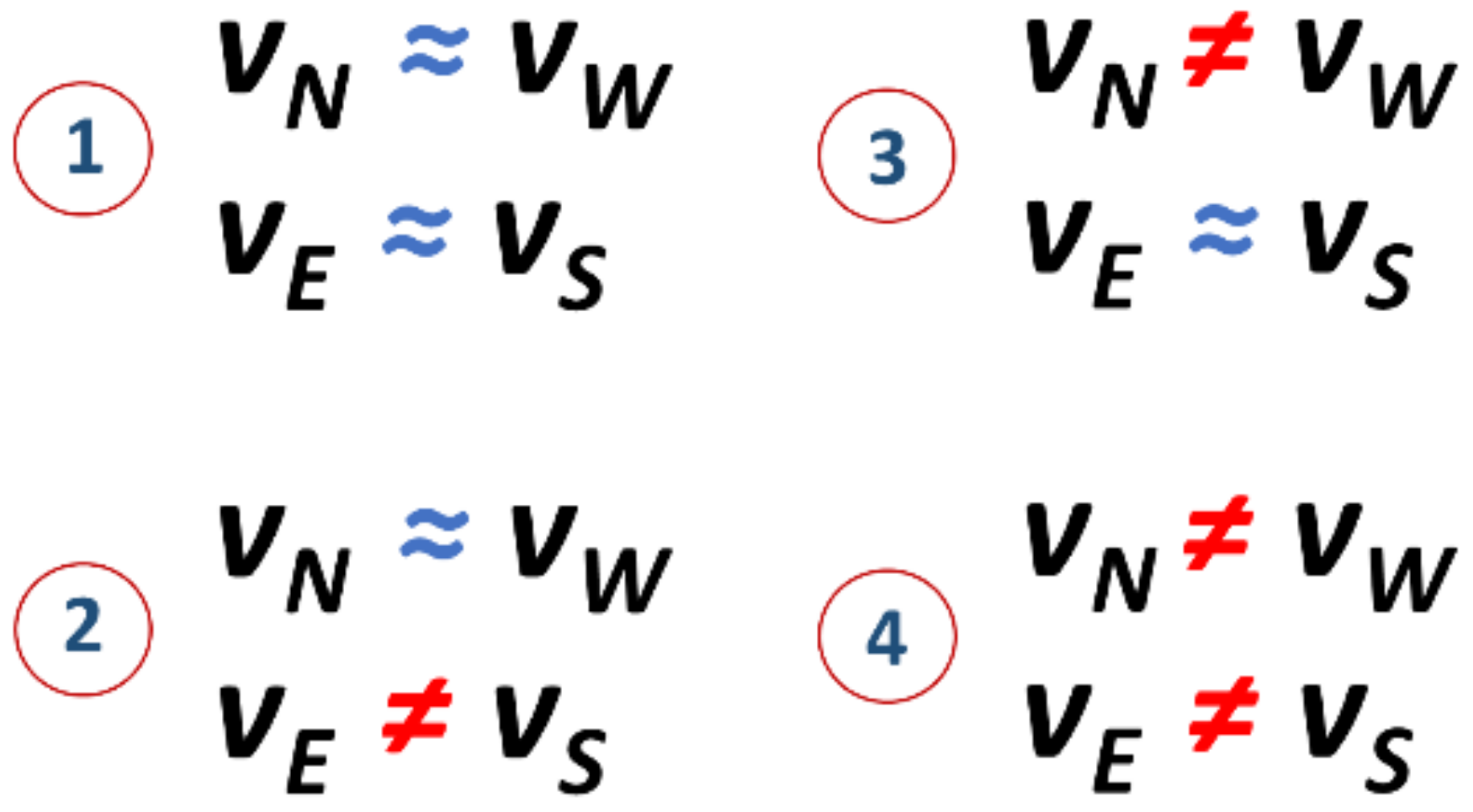
• Inlet velocity at N;
• Inlet velocity at W;
• Pressure at E outlet; and,
• Pressure at S outlet.

The velocity values (Table 2) are multiplied by the unit normal vector n, u = −vn, then, the input velocity is a vector of equal magnitude in the surface input boundary. The parameters k₀ and ε₀ must be defined, which are obtained from the Equations (8) and (9).

$$k_0=\frac{3}{2}{\left(v_0{I}_T\right)}^2$$

(8)

$${\epsilon }_0=\frac{C_{\mu }^{\frac{3}{4}}{k}^{\frac{3}{2}}}{L_T}$$

(9)

Turbulent intensity I_T (dimensionless) varies between 0.05 and 0.10. For the turbulent scale length, L_T (long unit) can be obtained according to the pipe radius r, obtaining 7% of it. L_T = 0.07r [39]. Therefore, the values were fixed on I_T = 0.05 and L_T = 0.07 × 0.0508 m = 0.003556 m.

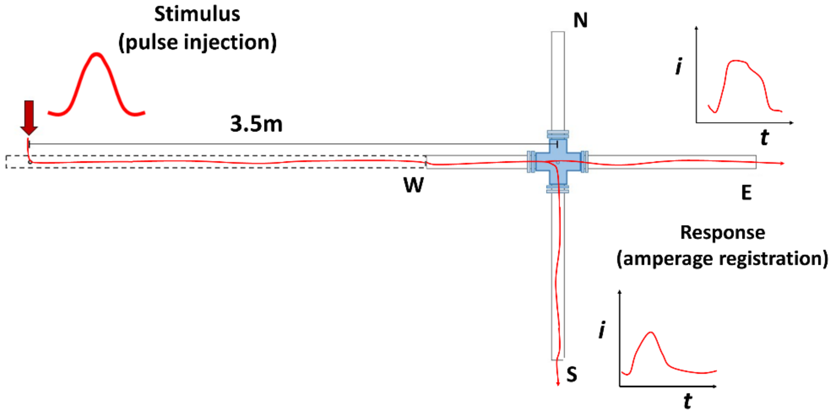
2.2.3. Residence Time Distribution

To sketch RTD curve in a fluid for transport of diluted species in dynamic regime, an averaged convection-diffusion equation for turbulent flow is used, Equation (10).

$$\frac{\partial C}{\partial t}=-\mathrm{u}·\nabla C+\nabla ·\left(D+D_T\right)\nabla C$$

(10)

where u is the velocity vector determined from Equation (2) of the hydrodynamic analysis, C is the tracer concentration, and D is the diffusion coefficient of the tracer. Under turbulent flow conditions, the concentration and the fluctuation parameters can be grouped in a turbulent diffusion term, D_T. This term can be evaluated considering the Schmidt Number (turbulent), Sc_T, for which, the equation proposed by Kays-Crawford [41] was used, Equations (11) and (12).

$$S{c}_T=\frac{{\mu }_T}{\left(\rho D_T\right)}$$

(11)

$$S{c}_T=\frac{1}{\frac{1}{2S{c}_{T\infty }}+\frac{0.3{\mu }_T}{\sqrt{S{c}_{T\infty }}\rho D}-{\left(0.3\frac{{\mu }_T}{\rho D}\right)}^2\left(1-exp\left(-\frac{\rho D}{0.3{\mu }_T\sqrt{S{c}_{T\infty }}}\right)\right)}$$

(12)

where Sc_T∞ is the value of Sc_T at a distance far from the wall, and it is fixed with a value Sc_T∞ = 0.85. It is considered to be a perfect mix at the tracer input boundary due to the distance with which it is injected.

The RTD curve is estimated by Equation (13) and it describes the distribution of the tracer through model at certain fixed time periods, from the injection of the tracer to the point of contact with the electrodes at outlets.

$$E\left(t\right)=\frac{C\left(t\right)}{{{\displaystyle \int }}_0^{\infty }C\left(t\right)dt}$$

(13)

where C (t) is the concentration that is time-dependent on time. The development of RTD curves was executed taking C (t) from the Equation (10).

Both DTR curves obtained, experimental and simulated will have different dimensions, so it is necessary to make a parameterization. A normalized function E ($\theta$) can be defined as [23]:

$$E\left(\theta \right)=\tau E\left(t\right)$$

(14)

where the dimensionless time $\theta$ is obtained by the spatial residence time $\tau$ = V/Q, V is the fluid volume of the model, and Q is the volumetric flowrate in each outlet.

The boundary and the initial conditions for solving the Equation (10) can be established as the tracer concentration, that is zero, C = 0, before the tracer injection in the reactor (t = 0) is performed. To simulate the tracer pulse injection, a mean form of the RTD is employed RTD at the outlets.

The mixing analysis was implemented in CFD, by the COMSOL Multiphysic software, 4.3b version in a computer of 64-bits operating system, Dual Core Xeon 2.30 GHz processor, and 96 GB of RAM. COMSOL has efficient simulation capabilities and complete graphic settings over other simulation commercial software packages [44]. This allows for better describing of different development patterns by function mathematical assignments in the simulation of tracer injection and the calculation of turbulent flow implemented in this study.

The discretization of the cross-junction volume was done using an unstructured mesh with tetrahedral, pyramid, and prism elements for simulation. According to the COMSOL manual [45], the mesh depends on the fluid flow and on the accuracy required. In many cases, the standard k-epsilon model with wall functions, that in this case, may deliver an accurate enough result at a much lower computational cost.

3. Results

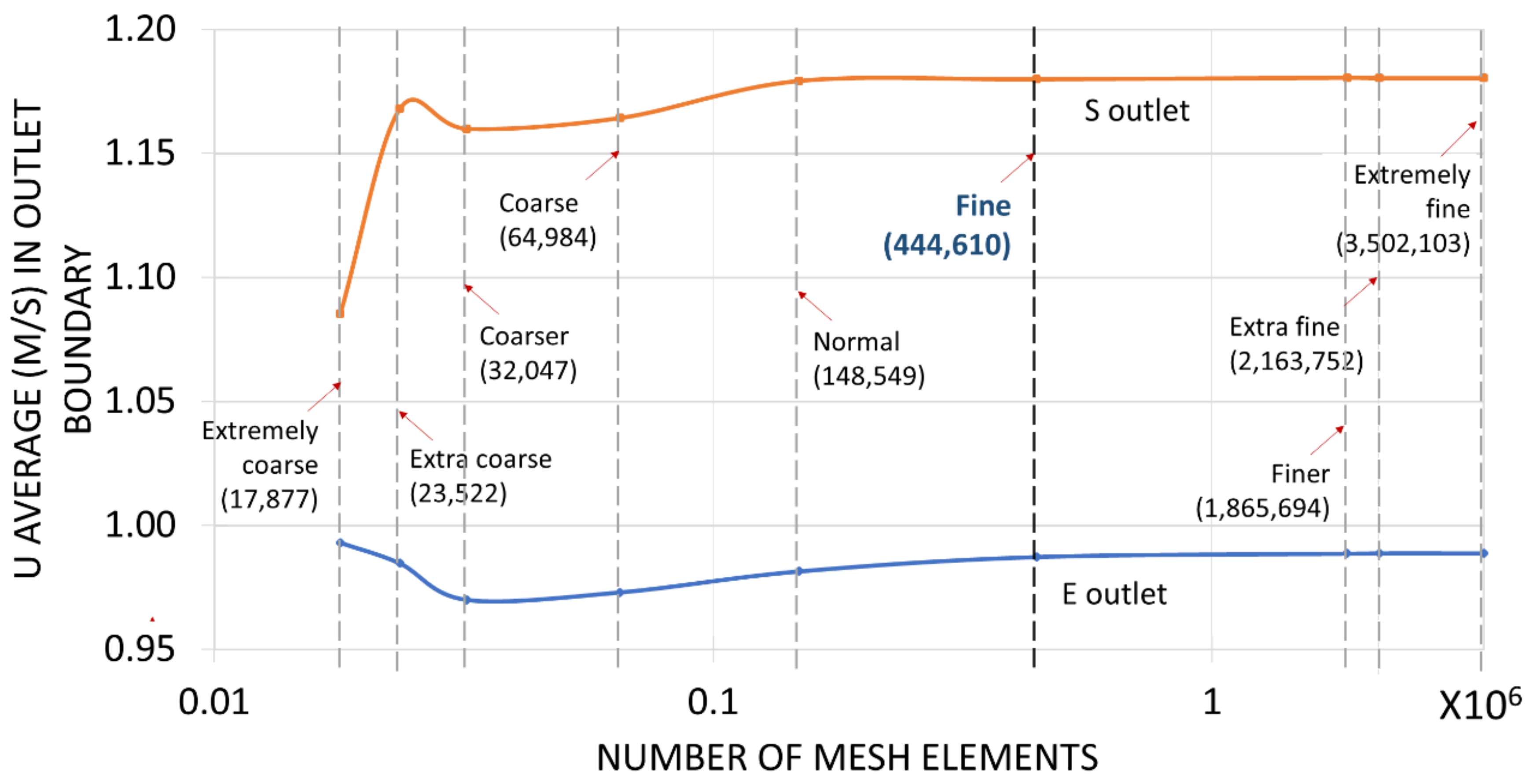
3.1. Mesh Selection and Sensibility Analysis

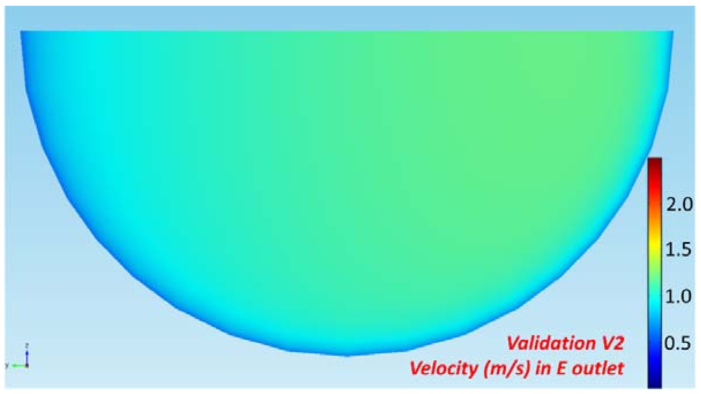
The COMSOL software already has predefined mesh grades for simulations in turbulent flow, varying only the mesh density degree. A sensitivity analysis (Figure 6) was carried out among nine different fineness degrees to determine which density is adequate for the numeric representation regarding the measurements that were made of pressure and velocity in the real experiment. Also, it is verified that by means of the value of y⁺ there is an adequate representation of the velocity profile.

The sensitivity analysis for scenario V1 is shown in Figure 6. For the degrees of coarse mesh (extremely coarse, extra coarser, coarser, coarse, and normal), the speed is having a variation for both outlets. However, from the FINE fineness level, besides the speeds adjusted and the increase of the degree of fineness, there is no other significant change. Therefore, the appropriate degree of mesh for the simulations is the FINE grade, it is conformed of 493,438 to 444,610 mesh elements, with the minimum and maximum edge lengths of 1.92, 0.362 cm, respectively; the number of elements depends on the drop of pressure that is generated from the experimental valves that control the flow that in the CFD was represented with an obstruction on the flow. Although only one case of sensitivity analysis is shown, it is not necessary to perform one for each scenario, since the geometry of the model varies insignificantly.

According to Veerstek & Malalasekera [38] and Moukalled, Margani & Darwish [46], y⁺ values in a range of (11.06 to 12.00) have important effects to turbulence production near the wall. As shown in the graph of Figure 6, the u velocity with respect to the mesh degree (by number of elements) stops varying from the FINE mesh degree. Therefore, this mesh degree was selected for the CFD model, which guarantees that the mesh tetrahedra established in the contours maintains a minimum y⁺ value of 11.1 (those were verified plotting values of y⁺ in a mesh graphic). The wall roughness was assumed to have a negligible effect. The solver that was employed was iterative, a generalized minimal residual, and a relative tolerance of accuracy of the CFD simulations considered a convergence criterion below 1 × 10⁻⁵. The typical solution around these meshes elements was unchanged.

3.2. CFD Simulation

The tracer injection must be defined in CFD simulations. However, the internal geometry of the sphere valve for the injection is controlled manually, and because of that, it is very irregular and difficult to obtain a chemical input pattern. Therefore, an interpolation was made between the tracer curves obtained at the outputs of the cross-junction. With this, a tracer input average is obtained at the injection point, and with this, the simulation is performed.

In the

Table 3. Approximation errors between experimental and simulated tests.

		V1			V2			V3			V4
		Exp	CFD	% Error	Exp	CFD	% Error	Exp	CFD	% Error	Exp	CFD	% Error
P (bar)	N	1.88	1.893	0.670%	1.60	1.577	1.437%	1.57	1.578	0.502%	1.96	1.971	0.575%
	W	1.88	1.893	0.677%	1.60	1.576	1.478%	1.56	1.575	0.982%	1.96	1.971	0.557%
V (m/s)	E	1.005	0.987	1.720%	1.062	1.060	0.211%	1.040	1.044	0.381%	1.246	1.237	0.744%
	S	1.167	1.180	1.130%	1.324	1.322	0.133%	1.302	1.294	0.593%	0.427	0.422	1.192%

, it can be verified that the approximation between the experimental and CFD results has a significant proximity. For velocity values, the average error is 0.76% and the maximum value reached is 1.72%. The errors in terms of pressure are on average 0.80% on the N boundary and 0.92% on the W boundary. In part, pressure differences that are presented will have to do with the decimals with which the readings were recorded. The values in CFD have 16 decimals of floating point, while the oscilloscope used registers of an average value of signal, in a given time, with two decimals.

The velocity values that were obtained in CFD correspond to vectors of a velocity field solved in the Navier Stokes Equation (3) for turbulent flow (k-ε model). However, to obtain an average value, COMSOL can estimate averages in a specific area (Figure 7). The selected mesh (FINE grade) approached the area of a contour (the outlet) of the pipe with good approximation (0.641% with respect to the real geometry obtained by a circumference).

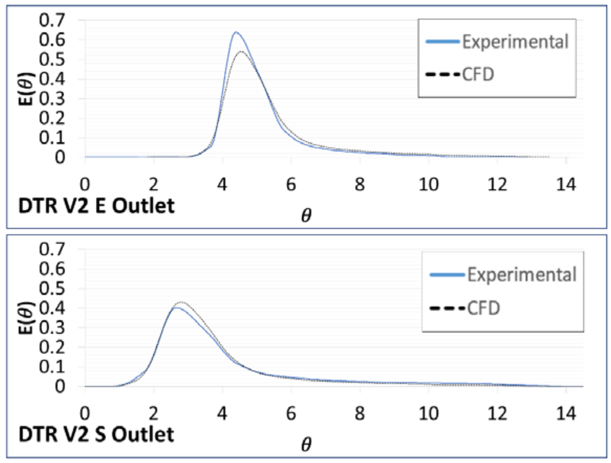
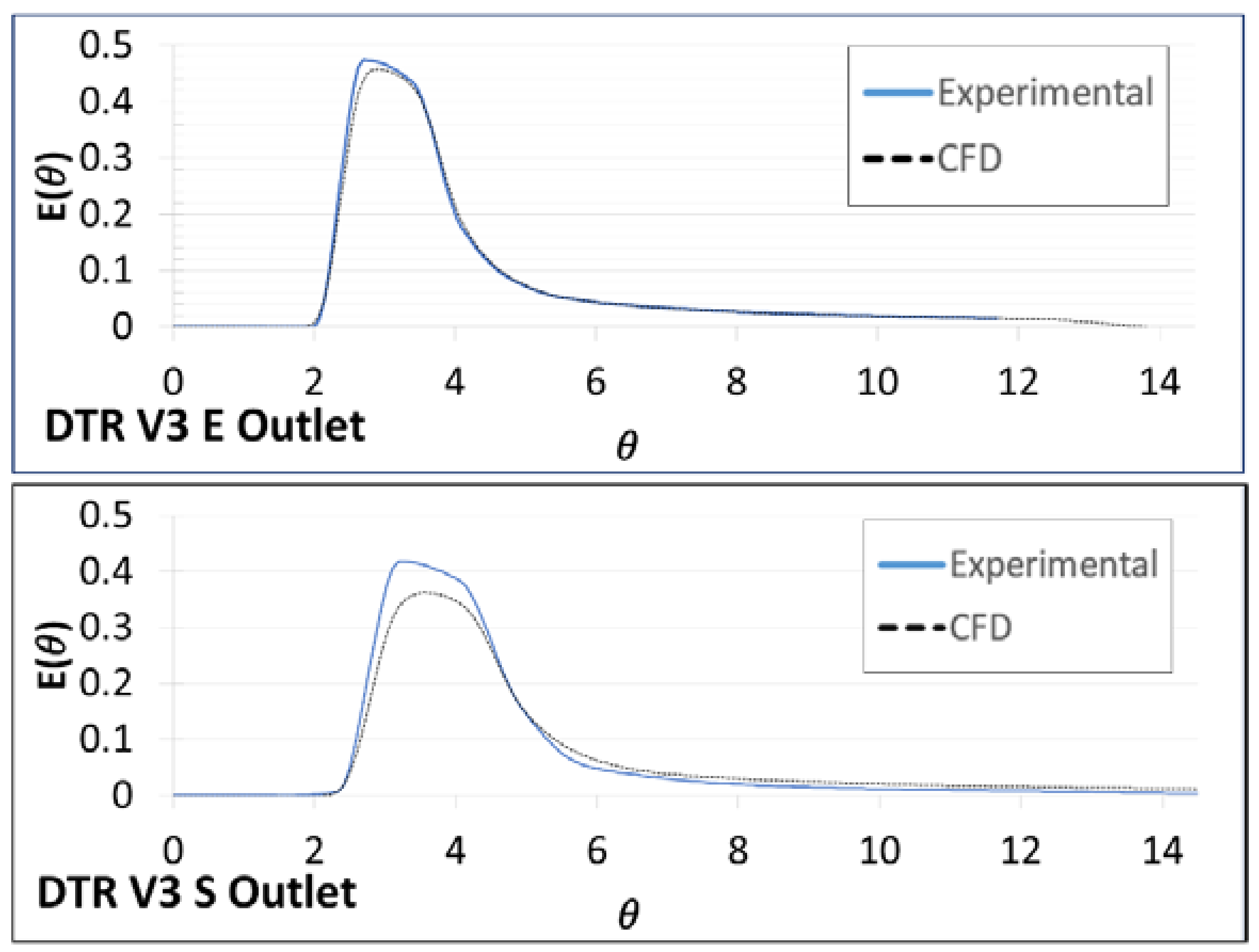
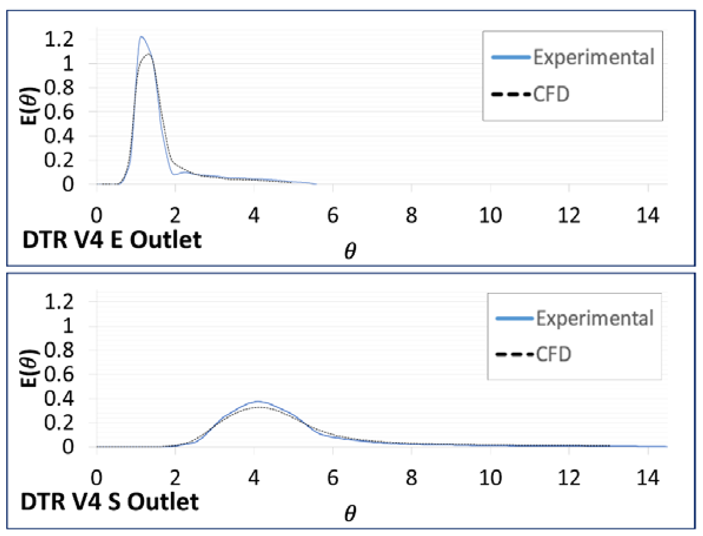
3.3. Residence Time Distribution Curves

Figure 8, Figure 9, Figure 10 and Figure 11 show the RTD curves, experimental and numerical, at different inlet velocities (V1 to V4). The current intensity value (milliAmperes), recorded in time intervals, varies by the exchange of copper ions in the electrode cells for the experimental RTD. On the other hand, the numerical RTD is the tracer concentration through time. The parameterization was made according to the Equation (14). It is important to emphasize that the CFD curves maintain a constant value most of the time, which is the stabilization of the received signal giving the supplied potential. Once the curves of the experimental and simulated tests are derived, a comparison is made between the curves to analyze the representation of the simulation. The dimensions of the axes of the graphs are: The dimensionless time (θ) on the horizontal axe and the normalized function for the concentration E (θ) on the vertical axe; in all the cases, there are diverse values indicating a not complete mixing. Close agreement between simulation and experimental tests were attained. The shape of the RTD curves evidences that the mixture in the pipe junctions does not obey a perfectly mixed model, owing to the fact that the maximum of the peak is far from θ = 0. The maximum of the curves was found at values of θ, higher than of the unity, what indicates that the fluid elements loss kinetic energy in the cross-junction due to the coalition of the hydrodynamic streams and the bifurcation of the fluid flow.

The variations between the experimental and theoretical RTD curves may be caused by the variability of the manual injection of the tracer, and tracer detection may be compared with the numerical convection-advection model on CFD. In almost all the cases, the peak of the experimental model is higher than in the CFD, resulting on the maximum concentration obtained in the experimental scenarios. Specially the Figure 11, where the RTD curve on the E outlet is too short when compared to the RTD curve on the S outlet, this is due to the outlet velocities that are registered on the experimental test, 1.25 m/s on the E outlet and 0.43 m/s on the S outlet, the tracer goes faster for the first velocity. The curves that were obtained for the validation tests V1 to V4 show that the tracer is following a tracer flow pattern that is similar to the experimental injection. To quantify these variations, an average error was calculated by the Root Mean Square Error (RMSE),

Table 4. Root Mean Square Error (RMSE) values for the four scenarios to evaluate variances in the RTD curves.

RMSE	V1	V2	V3	V4
E outlet	0.0215	0.0222	0.0093	0.0509
S outlet	0.0072	0.0109	0.0181	0.0140

.

Despite these differences, even the trend maintains a good proximity in terms of the distribution of the tracer, which shows that the proposed mathematical model is sufficiently calibrated model for describing the experimental mixture phenomenon in cross-junctions.

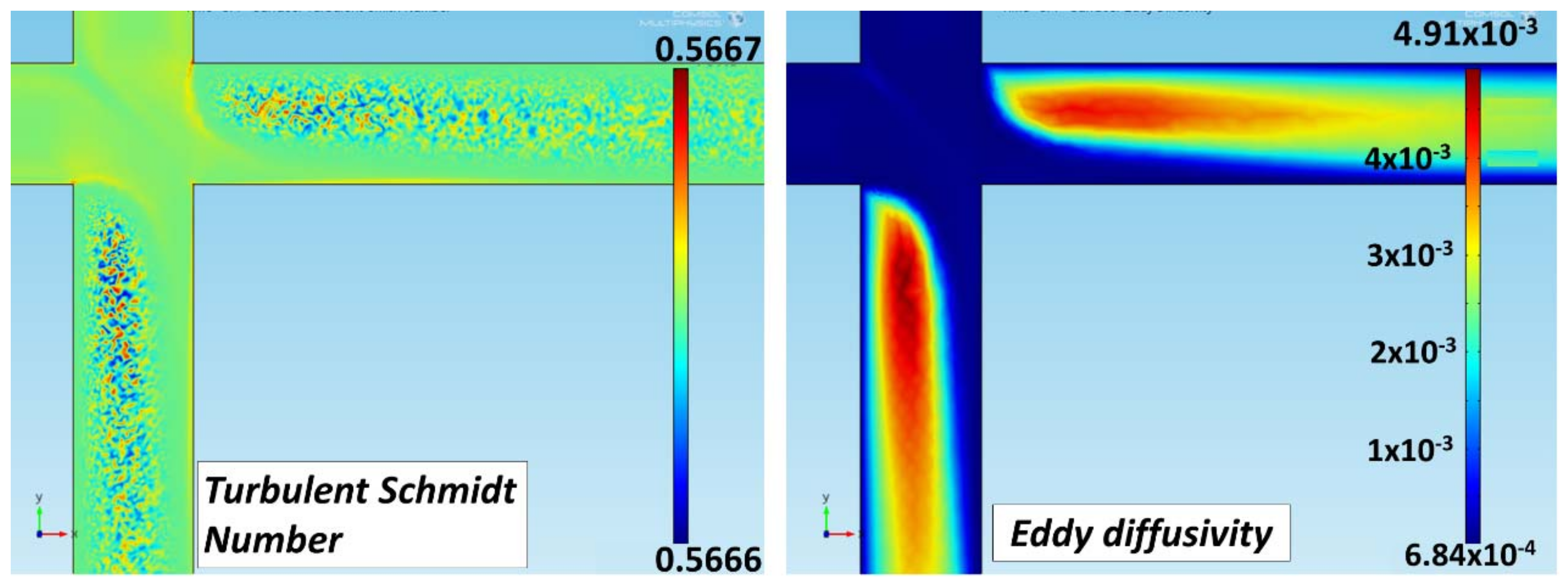
3.4. Variation of Sc_T Coefficient

A variation of the turbulent diffusivity is presented, in the search to verify if the model, under these conditions of pressure and velocity, varies significantly if the Sc_T coefficient is modified. The turbulent diffusivity was simulated in different values, using assignments to the Schmidt Turbulent Sc_T number. The range of values for this parameter is 0.61, 0.71, 0.81, and the value that was obtained by the Kays-Crawford model [41], which amounts to 0.5666.

The results indicate that the model is not sensitive to the variation of these Sc_T coefficients, since the parameterization of the curves reflects practically homogeneous results. This conclusion is verified, if a RMSE for each case is obtained again (

Table 5. Approximation of RTD curves varying Sc_T values.

RMSE	ScT (adim)
	0.61	0.71	0.81	K-C (0.566)
V1 E	0.0215	0.0216	0.0216	0.0215
V1 S	0.0073	0.0074	0.0076	0.0072
V2 E	0.0223	0.0226	0.02282	0.0220
V2 S	0.0109	0.0107	0.0106	0.0106
V3 E	0.0090	0.0085	0.0081	0.0093
V3 S	0.0182	0.0184	0.0186	0.0181
V4 E	0.0509	0.0509	0.0509	0.0509
V4 S	0.0143	0.0147	0.0151	0.0140

).

Table 5 shows that the variation is verified of the value used of Sc_T was based on the model of Kays-Crawford [41], and it was the most appropriate in most cases. The values of Sc_T have a very low impact in scale for the simulated model. In Figure 12, it is observed that the diffusion increases in the zones of greater recirculation, and there is less speed in the model. This should have a more significant influence, according to the bibliography. For the moment, it can be determined that the speed and pressure range far exceed the studied cases, and this tells us that at high levels of speed and pressure, the turbulent diffusivity does not have a significant impact on the transport of solute.

3.5. Incomplete Mixing Simulations

Once the CFD model has been calibrated, the mixing grade can be evaluated for diverse scenarios with the tracer injection at the two inlets, N and W. To represent the development of the mixing graphically, it was introduced by two parameters: Inlet relation (C_N/C_W); in the same way, Outlet relation (C_E/C_S). The diverse scenarios implemented were made by the combination of concentration at the inlets, in intervals of 0.25 mol/L, in a range Inlet relation = [0.00–2.00]. In the case of Inlet relation = 0.00, it means that C_N = 0.00 mol/L and C_W = 5 mol/L. At the same way, for an Inlet relation = 1.50, it means that C_N = 7.5mol/L and C_W = 5mol/L. The scenarios are represented in Figure 13, with the results for the outlet relation after the cross-junction mixing.

The four curves V1–V4 that are shown in Figure 13 represent the concentration relation between the two outlets E and S. Each curve (apparently straight lines) has different slopes. It can be observed that curves V1 and V2 have a similar development pattern, and are different from the curves V3 and V4. This is because V1 and V2 have closer input and output flow velocities, around 1 m/s for each one. However, curves V3 and V4 correspond to the input and output velocities with a wide degree of difference, between 0.427 to 1.302 m/s. This indicates that the transport of solute is by convective flow. This difference between velocities causes the tracer to flow at a higher rate at one output than at the other one. Therefore, the greater the difference between the input and output velocities, the greater the change in the slope of the generated curve.

Due to the behavior of the velocities mentioned above, the mixing behavior is maintained in a different proportion to the outlets in practically all of the cases. The complete mixing is not carried out on any scenario. Even the scenario with the same concentration in both inlets (Inlet Relation = C_N/C_W = 1) might not be a complete mixing. That is, since the result contains the same concentration at the inlets, it does not mean that a total mixture of the two incoming flows has been made. The complete mixing model assumes that “Outlet relation” must be equal to one in all cases, by the reason that the estimation assigns the same concentration at the two outlets. No one scenario has the behavior like a complete mixing.

4. Discussion and Conclusions

The physical characteristics of the experimental network, the pumping equipment, and the measuring devices used, allowed for achieving higher conditions of turbulence in the experimental model. To analyze the mixing that occurs in the cross-junction under these turbulence conditions, four scenarios were generated for flow velocities between 0.43 and 1.53 m/s; and for pressures around the cross-junction between 1.56 and 1.96 bar, we considered four kinds of similar velocities for the inlets and outlets boundaries around the cross-junction. It is common for these conditions to occur at these variations in real drinking water distribution networks.

The RTD curves present a novel and an adequate approximation, having RMSE values that are between 0.0072 and 0.0509. It means that the average distance of separation in some points of the curves carries this value. These separations occurred for the most part in the peaks of the curves. However, in the ascending and descending curvatures, they present a very precise similarity. In most of these regions, slopes are well represented, in all validation tests.

The variation of Sc_T solved many questions about the role of turbulent diffusion and the impact that it generates in these operating conditions. The RTD curves showed a minimal change between them. The change is almost inappreciable graphically. Therefore, more checks were obtained using the RMSE error for each curve, and the variation is seen up to the fourth decimal place of precision of the RMSE. This allows for concluding that convection is the main transport in diluted species, and that the diffusion does not affect much in the simulation of the tracer course through the cross-junction. Even with this, it was found that the model that was proposed by Kays-Crawford [41] was the adequate parameter when presenting the minimum RMSE values with respect to the turbulent Schmidt variation.

The mesh selection and the geometric construction were adequate, because the values that were derived from flow and average velocity in a contour surface correspond approximately to those that were calculated with analytical formulas. Also, the simulation times did not require extensive periods, and convergence was achieved without the presence of broken curves in the graphics. The graphics could be processed with a reasonable degree of affinity in the surface of symmetry. The hydrodynamic approach retains a low degree of error with respect to experimental measurements. The errors that were obtained at the inlet boundaries, for the pressure was between 0.502% to 1.478% on the four scenarios and at the outlets boundaries, for the velocity, was between 0.133% and 1.720%. It not only depended on the simulation in CFD and the mesh, but also on the continuity adjustments that were made in the experimental tests. These adjusted tests ensure that the entry costs were equivalent to the costs of exit in the trials, which was also kept in the CFD environment since one of the principles of its coding is based on the continuity equation for three dimensions.

Finally, the mixing grade that was evaluated for the scenarios with tracer injection at the two inlets, varying nine combinations, shows that the mixing behavior is maintained in a different proportion to the outlets in practically all the cases. This is due to the behavior of the velocities that are mentioned above; the complete mixing is not carried out on any scenario and it was verified with the RTD analysis, where they show us on the graphics of the RTD curves how the tracer was obtained on the outlet boundaries at different times and peaks. It also could be verified on the scenarios with the same concentration at the inlets, obtain the same concentration, but it does not mean that a total mixture of the two incoming flows has been made, and that was validated with the same RTD curves. No one of the scenario has any behavior like complete mixing.

References

1. Ahn, J.C.; Lee, S.W.; Choi, K.Y.; Koo, J.Y. Application of EPANET for the determination of chlorine dose and prediction of THMs in a water distribution system. Sustain. Environ. Res. 2012, 22, 31–38. [Google Scholar]
2. Shanks, C.M.; Sérodes, J.B.; Rodriguez, M.J. Spatio-temporal variability of non-regulated disinfection by-products within a drinking water distribution network. Water Res. 2013, 47, 3231–3243. [Google Scholar] [CrossRef] [PubMed]
3. Vasconcelos, J.J.; Rossman, L.A.; Grayman, W.M.; Boulos, P.F.; Clark, R.M. Kinetics of chlorine decay. Am. Water Works Assoc. 1997, 89, 54. [Google Scholar] [CrossRef]
4. Ozdemir, O.N.; Ucak, A. Simulation of chlorine decay in drinking-water distribution systems. J. Environ. Eng. 2002, 128, 31–39. [Google Scholar] [CrossRef]
5. Geldreich, E.E. Microbial Quality of Water Supply in Distribution Systems; CRC Press LLC: Boca Raton, FL, USA, 1996; ISBN 1-56670-194-5. [Google Scholar]
6. Knobelsdorf, M.J.; Mujeriego, S.R. Crecimiento bacteriano en las redes de distribución de agua potable: Una revisión bibliográfica. Ing. del Agua 1997, 4, 17–28. [Google Scholar] [CrossRef]
7. Alcocer-Yamanaka, V.H.; Tzatchkov, V.G.; Arreguín-Cortés, F.I. Modelo de calidad del agua en redes de distribución. Ing. Hidraul. Mex. 2004, 19, 77–88. [Google Scholar]
8. Rodríguez, M.J.; Rodríguez, G.; Serodes, J.; Sadiq, R. Subproductos de la desinfección del agua potable: Formación, aspectos sanitarios y reglamentación. Interciencia 2007, 32, 749–756. [Google Scholar]
9. Wang, W.; Ye, B.; Yang, L.; Li, Y.; Wang, Y. Risk assessment on disinfection by-products of drinking water of different water sources and disinfection processes. Environ. Int. 2007, 33, 219–225. [Google Scholar] [CrossRef] [PubMed]
10. Castro, P.; Neves, M. Chlorine decay in water distribution systems case study-lousada network. Electron. J. Environ. Agric. Food Chem. 2003, 2, 261–266. [Google Scholar]
11. Parks, S.L.I.; VanBriesen, J.M. Booster disinfection for response to contamination in a drinking water distribution system. J. Water Res. Plan. Manag. 2009, 135, 502–511. [Google Scholar] [CrossRef]
12. Tabesh, M.; Azadi, B.; Rouzbahani, A. Optimization of chlorine injection dosage in water distribution networks using a genetic algorithm. J. Water Wastewater 2011, 22, 2–11. [Google Scholar]
13. Kansal, M.L.; Dorji, T.; Chandniha, S.K.; Tyagi, A. Identification of optimal monitoring locations to detect accidental contaminations. In Proceedings of the World Environmental and Water Resources Congress 2012: Crossing Boundaries, Albuquerque, NM, USA, 20–24 May 2012; pp. 758–776. [Google Scholar]
14. Hernández, D.; Rodríguez, J.M.; Galván, X.D.; Medel, J.O.; Magaña, M.R.J. Optimal use of chlorine in water distribution networks based on specific locations of booster chlorination: Analyzing conditions in Mexico. Water Sci. Technol. Water Supply 2016, 16, 493–505. [Google Scholar] [CrossRef]
15. Weickgenannt, M.; Kapelan, Z.; Blokker, M.; Savic, D.A. Risk-based sensor placement for contaminant detection in water distribution systems. J. Water Res. Plan. Manag. 2010, 136, 629–636. [Google Scholar] [CrossRef]
16. Rathi, S.; Gupta, R. Monitoring stations in water distribution systems to detect contamination events. ISH J. Hydraul. Eng. 2014, 20, 142–150. [Google Scholar] [CrossRef]
17. Seth, A.; Klise, K.A.; Siirola, J.D.; Haxton, T.; Laird, C.D. Testing contamination source identification methods for water distribution networks. J. Water Res. Plan. Manag. 2016, 142. [Google Scholar] [CrossRef]
18. Xuesong, Y.; Jie, S.; Chengyu, H. Research on contaminant sources identification of uncertainty water demand using genetic algorithm. Cluster Comput. 2017, 20, 1007–1016. [Google Scholar] [CrossRef]
19. Montalvo, I.; Gutiérrez, J. Water quality sensor placement with a multiobjective approach. In Proceedings of the Congress on Numerical Methods in Engineering, Valencia, Spain, 3–5 July 2017. [Google Scholar]
20. Rathi, S.; Gupta, R. Optimal sensor locations for contamination detection in pressure-deficient water distribution networks using genetic algorithm. Urban Water J. 2017, 14, 160–172. [Google Scholar] [CrossRef]
21. Rossman, L.A. EPANET 2: User’s Manual; EPA/600/R-00/057; U.S. Environmental Protection Agency: Washington, DC, USA, 2000.
22. Sandoval, M.; Rosalba, F.; Walsh, F.C.; Nava, J.L.; Ponce de León, C. Computational fluid dynamics simulations of single-phase flow in a filter-press flow reactor having a stack of three cells. Electrochim. Acta 2016, 216, 490–498. [Google Scholar] [CrossRef] [Green Version]
23. Castañeda, L.F.; Antaño, R.; Rivera, F.F.; Nava, J.L. Computational fluid dynamic simulations of single-phase flow in a spacer-filled channel of a filter-press electrolyzer. Int. J. Electrochem. Sci. 2017, 12, 7351–7364. [Google Scholar] [CrossRef]
24. Rodríguez, I.L.; Valdés, J.A.; Alfonso, E.; Estévez, R.D. Dopico. Uso de técnicas estímulo—Respuesta para simular diagnósticos en esófago humano. In Proceedings of the Congreso Latinoamericano de Ingeniería Biomédica, La Habana, Cuba, 23–25 May 2001. [Google Scholar]
25. Van Bloemen Waanders, B.; Hammond, G.; Shadid, J.; Collis, S.; Murray, R. A comparison of Navier-Stokes and network models to predict chemical transport in municipal water distribution systems. In Proceedings of the World Water and Environmental Resources Congress, Anchorage, AK, USA, 15–19 May 2005; pp. 1–10. [Google Scholar]
26. Webb, S.W. High-fidelity simulation of the influence of local geometry on mixing in crosses in water distribution systems. In Proceedings of the ASCE World Water & Environmental Resources Congress, Tampa, FL, USA, 15–19 May 2007. [Google Scholar]
27. Ho, C.K.; Khalsa, S.S. EPANET-BAM: Water quality modeling with incomplete mixing in pipe junctions. In Proceedings of the Water Distribution Systems Analysis 2008 Conference, Kruger National Park, South Africa, 17–20 August 2008; pp. 1–11. [Google Scholar]
28. Song, I.; Romero-Gomez, P.; Choi, C.Y. Experimental verification of incomplete solute mixing in a pressurized pipe network with multiple cross-junctions. J. Hydraul. Eng. 2009, 135, 1005–1011. [Google Scholar] [CrossRef]
29. Liu, H.; Yuan, Y.; Zhao, M.; Zheng, X.; Lu, J.; Zhao, H. Study of Mixing at Cross-junction in Water Distribution Systems Based on Computational Fluid Dynamics. In Proceedings of the International Conference on Pipelines and Trenchless Technology, Beijing, China, 26–29 October 2011; pp. 552–561. [Google Scholar]
30. Romero-Gomez, P.; Lansey, K.E.; Choi, C.Y. Impact of an incomplete solute mixing model on sensor network design. J. Hydroinform. 2011, 13, 642–651. [Google Scholar] [CrossRef] [Green Version]
31. Yu, T.C.; Shao, Y.; Shen, C. Mixing at cross joints with different pipe sizes in water distribution systems. J. Water Res. Plan. Manag. 2014, 140, 658–665. [Google Scholar] [CrossRef]
32. Shao, Y.; Yang, Y.J.; Jiang, L.; Yu, T.; Shen, C. Experimental testing and modeling analysis of solute mixing at water distribution pipe junctions. Water Res. 2014, 56, 133–147. [Google Scholar] [CrossRef] [PubMed]
33. Mompremier, R.; Pelletier, G.; Mariles, Ó.A.F.; Ghebremichael, K. Impact of incomplete mixing in the prediction of chlorine residuals in municipal water distribution systems. J. Water Supply Res. Technol. 2015, 64, 904–914. [Google Scholar] [CrossRef]
34. Mckenna, S.A.; O’hern, T.; Hartenberger, J. Detailed Investigation of Solute Mixing in Pipe Joints Through High Speed Photography. Water Distrib. Syst. Anal. 2008, 1–12. [Google Scholar] [CrossRef]
35. Ho, C.K.; O’Rear, L., Jr. Evaluation of solute mixing in water distribution pipe junctions. Am. Water Works Assoc. J. 2009, 101, 116. [Google Scholar] [CrossRef]
36. Choi, C.Y.; Shen, J.Y.; Austin, R.G. Development of a comprehensive solute mixing model (AZRED) for double-tee, cross, and wye junctions. Water Distrib. Syst. Anal. 2008, 1–10. [Google Scholar] [CrossRef]
37. Gualtieri, C.; Jiménez, P.L.; Rodríguez, J.M. A comparison among turbulence modelling approaches in the simulation of a square dead zone. In Proceedings of the 19th Canadian Hydrotechnical Conference, Vancouver, BC, Canada, 9–14 August 2009. [Google Scholar]
38. Versteeg, H.K.; Malalasekera, W. An Introduction to Computational Fluid Dynamics: The Finite Volume Method; Pearson Education: New York, NY, USA, 2007. [Google Scholar]
39. Rosales, M.; Pérez, T.; Nava, J.L. Computational fluid dynamic simulations of turbulent flow in a rotating cylinder electrode reactor in continuous mode of operation. Electrochim. Acta 2016, 194, 338–345. [Google Scholar] [CrossRef]
40. Hanjalic, K. Two-Dimensional Asymmetric Turbulent Flow in Ducts. Ph.D. Thesis, University of London, London, UK, 1970. [Google Scholar]
41. Kays, W.M.; Crawford, M.E.; Weigand, B. Convective Heat and Mass Transfer; McGraw-Hill Education: New York, NY, USA, 2005. [Google Scholar]
42. Martinez-Solano, F.J.; Iglesias-Rey, P.L.; Gualtieri, C.; López Jiménez, P.A. Modelling flow and concentration field in rectangular water tanks. In Proceedings of the International Environmental Modelling and Software Society (iEMSs), Ottawa, ON, Canada, 5–8 July 2010. [Google Scholar]
43. Moncho-Esteve, I.J.; Palau-Salvador, G.; López Jiménez, P.A. Numerical simulation of the hydrodynamics and turbulent mixing process in a drinking water storage tank. J. Hydraul. Res. 2005, 2, 207–217. [Google Scholar] [CrossRef]
44. Georgescu, A.M.; Georgescu, S.C.; Bernad, S.; Coşoiu, C.I. COMSOL Multiphysics versus Fluent: 2D numerical simulation of the stationary flow around a blade of the Achard turbine. In Proceedings of the 3rd Workshop on Vortex Dominated Flows, Timisoara, Romania, 1–2 June 2007. [Google Scholar]
45. COMSOL. CFD Module User’s Guide; Version 4.3bCOMSOL Multiphysics; COMSOL, Inc.: Burlington, MA, USA, 2013. [Google Scholar]
46. Moukalled, F.; Mangani, L.; Darwish, M. The Finite Volume Method in Computational Fluid Dynamics; Springer: Berlin, Germany, 2016; Volume 113. [Google Scholar]
Figure 1. Cross-junction boundaries. The distances correspond to the pressure registration points.
Water 10 00733 g001
Figure 2. Equipment to measure flow (electromagnetic: (a,c), propeller volumetric: (b,d)) and pressure around the cross-junction (oscilloscope and pressure transducer: (e)).
Water 10 00733 g002
Figure 3. Tracer injection and registration points.
Water 10 00733 g003
Figure 4. Equipment for stimulus-response technique.
Water 10 00733 g004
Figure 5. Boundary velocities for experiments.
Water 10 00733 g005
Figure 6. Mesh sensibility analysis.
Water 10 00733 g006
Figure 7. Example of a velocity contour plot.
Water 10 00733 g007
Figure 8. Residence Time Distribution (RTD) curves for V1.
Water 10 00733 g008
Figure 9. RTD curves for V2.
Water 10 00733 g009
Figure 10. RTD curves for V3.
Water 10 00733 g010
Figure 11. RTD curves for V4.
Water 10 00733 g011
Figure 12. ScT and eddy diffusivity plots based on the Kays-Crawford [41] model (Equation (12)). High values appear in the turbulent flow zones.
Water 10 00733 g012
Figure 13. Solute mixing for variable concentration at the inlets.
Water 10 00733 g013