Calibration Parameter Selection and Watershed Hydrology Model Evaluation in Time and Frequency Domains


Department of Watershed Sciences, Utah State University, Logan, UT 84322-5210, USA
*
Author to whom correspondence should be addressed.
Water 2018, 10(6), 710; https://doi.org/10.3390/w10060710
Submission received: 11 April 2018
/
Revised: 29 May 2018
/
Accepted: 29 May 2018
/
Published: 31 May 2018
(This article belongs to the Section Hydrology)
Abstract
:Watershed scale models simulating hydrological and water quality processes have advanced rapidly in sophistication, process representation, flexibility in model structure, and input data. With calibration being an inevitable step prior to any model application, there is need for a simple procedure to assess whether or not a parameter should be adjusted for calibration. We provide a rationale for a hierarchical selection of parameters to adjust during calibration and recommend that modelers progress from parameters that are most uncertain to parameters that are least uncertain, namely starting with pure calibration parameters, followed by derived parameters, and finally measured parameters. We show that different information contained in time and frequency domains can provide useful insight regarding the selection of parameters to adjust in calibration. For example, wavelet coherence analysis shows time periods and scales where a particular parameter is sensitive. The second component of the paper discusses model performance evaluation measures. Given the importance of these models to support decision-making for a wide range of environmental issues, the hydrology community is compelled to improve the metrics used to evaluate model performance. More targeted and comprehensive metrics will facilitate better and more efficient calibration and will help demonstrate that the model is useful for the intended purpose. Here, we introduce a suite of new tools for model evaluation, packaged as an open-source Hydrologic Model Evaluation (HydroME) Toolbox. We apply these tools in the calibration and evaluation of Soil and Water Assessment Tool (SWAT) models of two watersheds, the Le Sueur River Basin (2880 km2) and Root River Basin (4300 km2) in southern Minnesota, USA.
1. Introduction
1.1. Hydrologic Models and the Calibration Challenge
Watershed scale models simulating hydrology and water quality have evolved considerably over the past few decades. Such models are essential to inform policy and management decisions at scales ranging from individual farm fields to the entire Mississippi River Basin [1]. Watershed hydrology models, such as the Soil and Water Assessment Tool (SWAT), Water Erosion Prediction Project (WEPP) and Gridded Surface Subsurface Hydrologic Analysis (GSSHA) have advanced rapidly in sophistication, process representation and flexibility regarding model components and input data. The caveat that accompanies this sophistication and flexibility is that each process is often represented by multiple adjustable parameters, which greatly increases the challenge of calibration and problem of equifinality [2,3,4]. In the spirit of continued advancement, this paper examines current techniques and metrics used to evaluate hydrologic models for the purpose of calibration and validation and proposes several additional techniques to improve quantitative evaluation of models.
Calibration is the process of estimating model parameter values to enable a hydrologic model to match observations [5] such as streamflow. While calibration cannot necessarily circumvent more fundamental problems associated with model structure, data availability, and initial and boundary conditions, some form of calibration is necessary to improve reliability for most distributed hydrologic model applications [6]. Over the past few decades, numerous publications have highlighted the challenges associated with calibration such as; physical distortion by tuning incorrect parameters, inability of performance measures used in calibration to capture all aspects of the hydrologic times series, and limitations in the search schemes, such as Monte Carlo Markov Chain, uniform Monte Carlo or Latin Hypercube [7,8,9,10]. Several techniques have been proposed to partially resolve some of these challenges [5,6].
While the theoretical underpinnings of calibration have advanced considerably [11], several key challenges persist. Challenges stem from the sheer number and complexity of processes involved, many of which are non-linear, exhibit interdependencies, and are subject to large variability in both time and space. Automatic calibration procedures have become common for watershed hydrology models as manual calibration needs considerable expertise with the model. Gathering more and higher-resolution data will not fully resolve calibration issues, as many parameters are conceptual representations of abstract physical processes and therefore cannot be measured [5]. In other words, the non-uniqueness problem can potentially be reduced, but not eliminated, with more data. Notwithstanding the challenges in calibration itself, calibration should not be substituted for proper model setup and choice of appropriate input datasets as demonstrated by [4,12]. Further, the importance of using appropriate datasets, such as local weather data in contrast to global datasets to achieve adequate calibration was demonstrated by [13].
We introduce several new tools to improve model evaluation, packaged as the Hydrologic Model Evaluation (HydroME) Toolbox, which is freely available for download from https://qcnr.usu.edu/labs/belmont_lab/resources or https://github.com/Kkumarasamy/HydroME. HydroME is a general purpose (model independent) post processing tool written in MATLAB with the ability to process and compare time series. Other tools that can aid in the calibration of hydrologic models already exist, such as; HydroGOF [14], HydroTest [15], FITEVAL [16] and Water Engineering Time Series PROcessing tool (WETSPRO) [17,18,19]. These tools generate central tendency values of time domain model performance metrics. HydroME, however, generates model performance metrics and graphics in both time and frequency domains. Additionally, HydroME also helps to identify parameters that should be considered for calibration.
We utilize SWAT throughout this paper because it has emerged as a leading model for informing policy and management. SWAT benefits from an enormous user and developer base that has struck a synergistic balance of encouraging grassroots innovation and adaptation [20], while maintaining model stability and version control. In many ways, it is a Community Hydrologic Model called for by [21]. In 2015 alone, 437 journal articles were published based on the SWAT model [22]. However, we note that the tools and approach we take are more broadly applicable to any watershed hydrology model.
1.2. Model Evaluation and Reporting Measures
We propose that the discipline of hydrologic modeling is sufficiently mature to adopt a new suite of model performance metrics that more specifically and meaningfully convey the suitability of a model to answer the questions of interest. The increasingly interdisciplinary nature of hydrology and wide-ranging use of hydrologic models to make predictions about water quality, sediment transport, ecological processes and ecosystem health increase the urgency for more targeted and robust measures of model performance.
Lumped metrics such as Nash Sutcliffe Efficiency (NSE), coefficient of determination (R2) and percent bias (PBIAS) have been established as key model performance benchmarks [23,24,25]. These metrics provide an averaged measure of error and are intentionally biased towards large magnitude flows [26]. NSE is slightly better than R2 for many model applications as it is sensitive to the observed and model simulated means and variances [27]. It is important to note, however, that these metrics only address magnitude errors and are insensitive to critical flow thresholds that may be important to answer the questions of interest. Limitations of NSE are reported in several studies [26,28,29]. Many other streamflow characteristics may be important, depending on whether your model is being used to simulate water, sediment or nutrient fluxes or aquatic habitat quality [30,31,32]. Increasingly, watershed hydrology models are used for predictions, or as inputs to other models with processes operating at daily and sub-daily time steps. In such cases, models evaluated at monthly scales are of limited value. Further, streamflow event structures are not characterized by these metrics. For example, NSE and R2 are ambiguous as to shape of streamflow hydrograph from an individual storm. The goal of this paper is to provide insight and new tools that facilitate meaningful model evaluation throughout the process of calibration, validation and communication of results.
2. Study Area and Model Setup
We illustrate our approach using two carefully selected case studies. The contrasting environments represented by our study watersheds challenge the model structure in different ways and present distinct calibration challenges.
2.1. Le Sueur River Basin (LSRB)
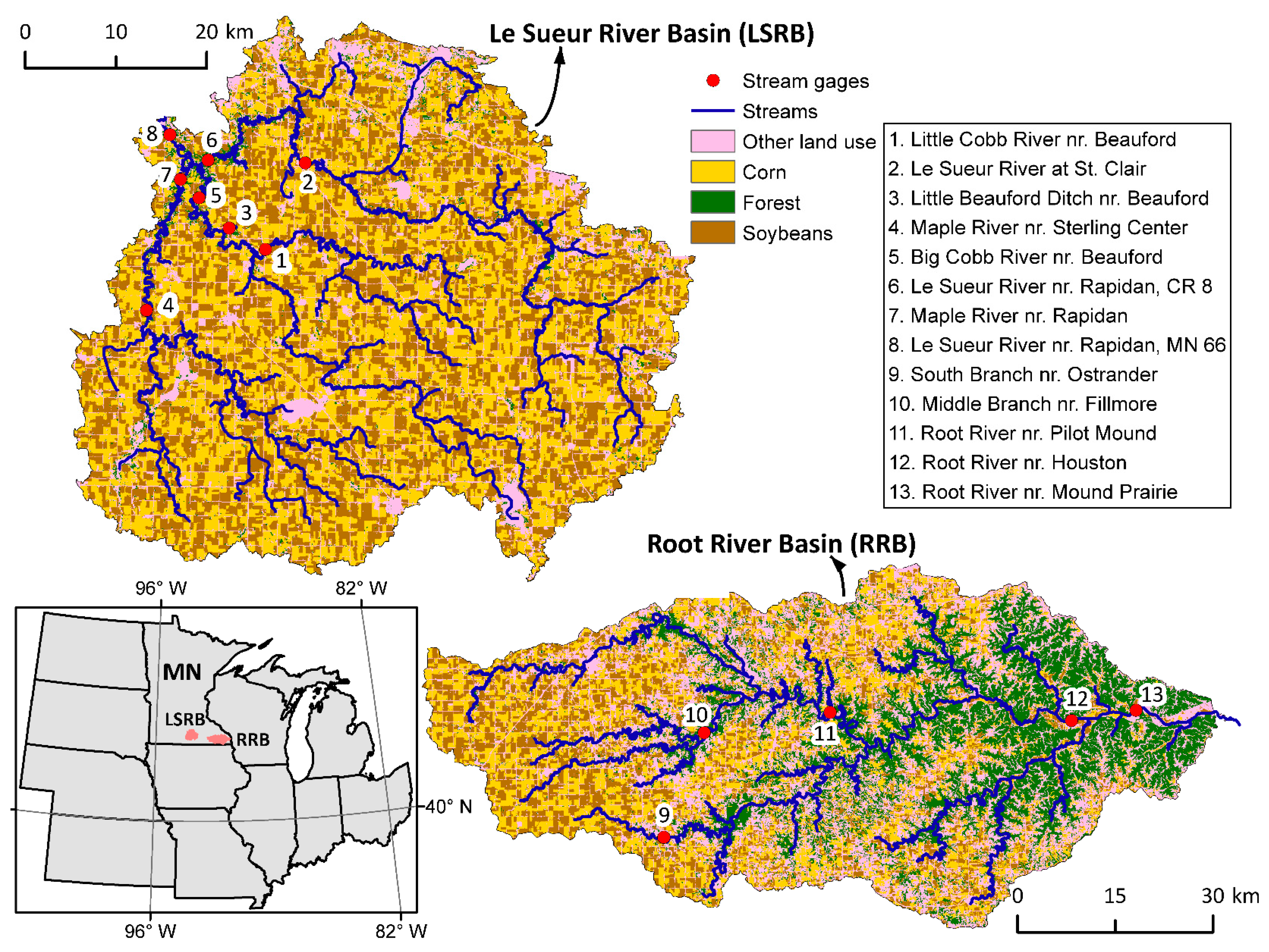
The 2880 km2 LSRB in south-central Minnesota shown in Figure 1 is listed as impaired for excessive sediment and nutrients and is implicated as a primary contributor to water quality problems in the Minnesota River and Lake Pepin on the Mississippi River [33,34,35,36]. The dominant land use consists of Corn and Soybean in LSRB and covers approximately 80% of the watershed area as shown in Figure 1. Humans have profoundly altered the sub-surface hydrology with an extensive network of drain tiles (corrugated plastic tubing installed 30–100 cm below the soil surface) [36,37]. ArcSWAT 2012.10.1.15 for ArcGIS 10.1 was used to extract SWAT text files using 10 m DEM for topography [38,39], USDA Cropland Data Layer (CDL) for land use [40] and Soil Survey Geographic Database (SSURGO) data for soils [41]. Temperature (maximum and minimum) and precipitation data were obtained from [42] at 4 km resolution and averaged daily within each of the 175 sub-basins. Solar radiation and relative humidity data were obtained from global weather data for SWAT [43]. Hydrologic Response Units (HRUs) were defined using the multiple HRUs option with 5% for land use, 15% for soil and 10% for slope. Corn, soybean and wetlands were exempted from the land use threshold definition resulting in 1823 HRUs for the basin. Management practices implemented in the model are shown in Figure S1 in Supplementary Information (SI). More information about the LSRB SWAT model is provided in Section S1 of the SI.
A multipoint and multi-parameter calibration was employed, and the model was calibrated and validated against daily streamflow at 8 gages within the basin. A split sample approach was employed by dividing streamflow record at each of the eight gages into calibration and validation datasets. The term validation is used to remain consistent with the rest of the literature and does not imply that the watershed model can be fully validated. Base flow was separated from the calibration period flow data using the Baseflow filter program to initialize the ALPHA_BF parameter [44,45]. However, the initialized value of the parameter ALPHA_BF was replaced with the ranges specified in Table S1 during calibration as the model could not otherwise be calibrated to a satisfactory degree. All parameters selected for calibration and their calibrated values are listed in Table S1 in SI and details of partitioning streamflow into calibration and validation data in Table S3. Table S1 also shows how each of the parameters were classified during calibration based on the parameter classification approach described in Section 3.4. Streamflow measurements at upstream gages were calibrated first, followed by downstream gages using three goodness of fit metrics: (1) NSE, (2) R2 and (3) PBIAS. A brief description of these three metrics provided in Section S2 of the SI.
2.2. Root River Basin (RRB)
The 4300 km2 RRB in southeastern Minnesota shown in Figure 1 is also listed as impaired for excess sediment and nutrients under the USEPA Clean Water Act [46]. The upper third of the basin is flat and underlain by fine-grained glacial till. The majority of the lower two-thirds of the basin is dominated by hundreds of caves and sinkholes connecting surface flow paths to the poorly mapped karst groundwater network. Topography of this zone is characterized by relatively steep, forested hillslopes with row crop agriculture and pasture on lower sloped terrain. The geologic, geomorphic and hydrologic setting of the Root River provides a useful contrast to the Le Sueur watershed for our discussion of model calibration and evaluation.
The RRB SWAT model uses the SWAT2012.exe Revision 622 packaged with ArcSWAT 2012.10_1.15. Subbasin delineation is accomplished using 10 m topography data, by choosing a threshold-based stream definition and by specifying locations where a model output is required to facilitate comparison with measured streamflow. The threshold-based streamflow definition option allows us to control the size of the subbasins, which is crucial for capturing variability in precipitation and also to simulate flows at any desired location where flow outputs are needed. The RRB model was built using the multiple HRUs definition option by specifying a threshold of 20% for land use, 0% for soils, and 0% for slope, resulting in 17,174 HRUs. Topography, soils, and land use data were obtained from same sources as LSRB. Management practices implemented are shown in Figure S2 in SI.
Karst presents a model structure limitation, as SWAT does not explicitly model preferential flow pathways. However, SWAT is commonly applied to such watersheds [47] with lumped treatment of such flow pathways. RRB model was initialized with land use data from 2006, which is the first year when the CDL was available for Minnesota. Details on how this information was compiled is described in [48]. Hydrologic effects of the karst system (i.e., stream flow loss or gain) were represented by altering tributary and main channel transmission losses. Rapid and slow responses of groundwater contribution to streamflow that result from preferential pathways were accomplished by altering groundwater delay times and rate and quantity of groundwater that is fed to streamflow. Similar to the LSRB SWAT model, a multipoint and multi-parameter calibration was employed, and the model was calibrated and validated against daily streamflow at 5 gages within the basin. A split sample approach was employed by dividing the streamflow record at each of the five gages into calibration and validation datasets similar to LSRB SWAT model. Base flow was separated from the calibration period flow data using the Baseflow filter program to initialize the ALPHA_BF parameter [44,45]. However, the initialized value of the parameter ALPHA_BF was replaced with the ranges specified in Table S3 during calibration as the model could not be calibrated using the values predicted by the Baseflow filter program. More information about the RRB SWAT model is provided in Section S1 of the SI. All the model parameters that were calibrated are listed in Table S3 and details of partitioning streamflow into calibration and validation data in Table S4 of the SI. The LSRB and RRB SWAT models are available for download at https://github.com/Kkumarasamy/Models.
3. Parameter Choice, Estimation, and Classification
3.1. Parameter Choice Problem
Choosing which parameters to adjust in a complex watershed hydrology model such as SWAT can be a daunting task. Any given parameter can be sensitive within a particular range and during specific seasons or time periods. Further, the sensitivity of any given parameter may vary depending on one or multiple other parameter values. How should one choose which parameters to adjust in a complex model such as SWAT, with over 100 potentially adjustable parameters to choose from? More importantly, when one achieves what is deemed to be a good or acceptable calibration, how can they be confident that they have achieved high performance metrics for the right reasons and have not mathematically distorted the physical system in ways that may bias their results or interpretations? Motivated by these shortcomings implicit in the blind (nondiscriminatory or considering only process and not uncertainty in the data) tuning of parameters we propose general guidelines for selection of parameters for calibration by grouping parameters into different categories as described in Section 3.4.
3.2. Fully Automated and Intervention Type Calibration Procedures
Automated calibration and other hybrid procedures have become increasingly common over the past decade [49,50,51]. The objective nature of automated parameter adjustment makes these approaches very appealing. Indeed, these approaches offer many advantages and will become increasingly effective as techniques and algorithms improve. However, these procedures typically rely, often exclusively, on a single lumped closeness measure, such as Root Mean Square Error (RMSE) [29] or the R2 [52]. As described in [5] and discussed above, a single criterion is inherently predisposed to bias towards certain components of the hydrologic time series. Automated procedures will be improved by the use of multiple evaluation criteria as discussed here and by [11]. However, even a multicriteria approach may not resolve the issue as described in Section S3 of the SI. Further, automated procedures adjust parameter values without regard for process, time periods when they are sensitive, or physical meaning of any given combination. Although automation can help the calibration process become more objective, efficient and practical, these procedures are not a panacea substitute for expert hydrologic intuition and understanding.
3.3. Parameter Selection Based on Sensitivity
Whether automated or manual calibration is used, a common approach is to adjust the parameters that display the highest sensitivity [9,53,54]. This approach is attractive because improvements in calibration can be achieved with a minimal number of adjustments. However, sensitivity alone should not be the criterion for parameter set selection for calibration, because the most sensitive parameter is not necessarily the one causing the divergence between the modeled and measured values (See Section S3 of the SI, where calibration can be achieved through many different parameter combinations). Parameter sensitivity in this paper is defined as the change in outcome (e.g., a given streamflow metric) in response to a specified change in a parameter value. If there is a large deviation between the pre- and post-parameter change curves, we consider the parameter to be sensitive. For example, CN2 is a highly sensitive parameter and thus minor adjustments can drastically alter the hydrograph. For this reason, CN2 is commonly used as a “sledge hammer” in calibration to make significant changes across a wide range of flow values in an effort to achieve a higher performance metric value [55], regardless of whether or not there is reason to believe modified CN2 are justifiable. Thus, CN2 is a very sensitive parameter, but there may not be a physical basis for its inclusion as a calibration parameter. Section S4 of the SI illustrates this conundrum, where we have varied CN2 ±10% and show the corresponding stream flow outcome for 1000 runs for the South Branch gage in the RRB.
3.4. Parameter Classification
Calibration can be defined as an ill-posed, non-linear inverse problem that can lead to non-unique solutions, with the outcome to parameter mapping being non-unique. Here we present a rationale to determine parameters that can serve as suitable candidates for calibration based on how much information we have about a particular parameter. Our reasoning for including only a subset instead of all 1000+ parameters is based on whether the parameters were measured, derived from data, or constrained solely through a calibration exercise. It is worthwhile to reiterate the importance of utilizing the best available data prior to adjusting parameters to achieve desired performance metrics [4,12].
To address challenges with parameter choice, whether using manual or fully automated procedures and in the time or frequency domain, we emphasize that the modeler consider different classes of parameters. Our approach attempts to choose the most relevant and parsimonious set of parameters to guide calibration, minimize physical distortion of the hydrologic system being modeled, focus calibration and validation on relevant hydrologic metrics, and reduce the problem of equifinality. Other approaches such as posing the calibration problem using Bayesian concepts exist [56]. We have taken an approach to address calibration parameter uncertainty in a simple way by means of separating the parameters to include/exclude for calibration in sequential order. Additionally, the number of parameters is continuously increasing in distributed hydrologic models to describe new processes. Thus, posing the calibration problem by assigning probability density functions (pdf’s) to each parameter will be a challenge as much of the information may not be available for all watersheds. The approach presented here is qualitative and does not require a prior pdf specification. We wanted to illustrate an approach that does not need additional information and can be an alternative to other approaches.
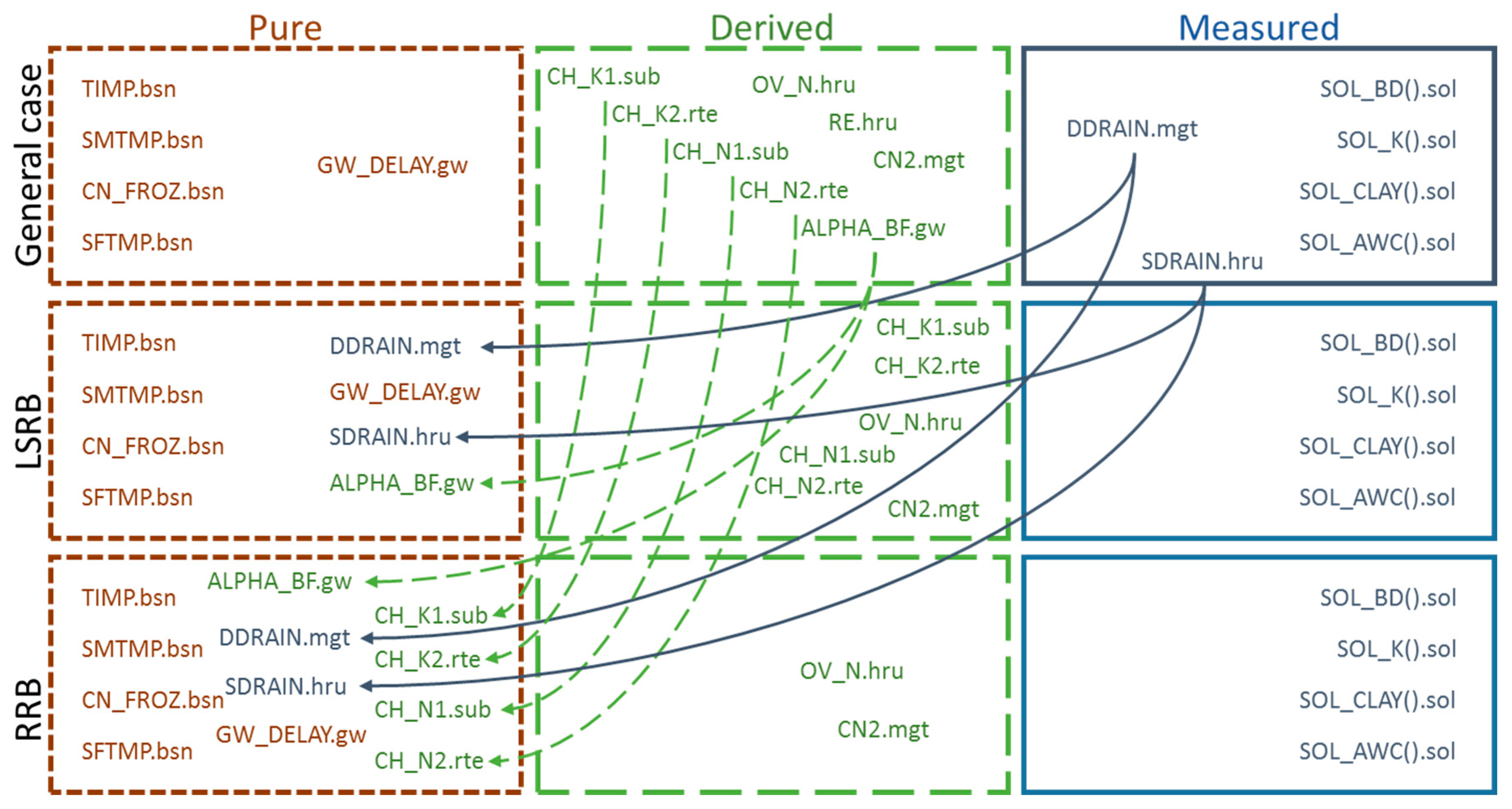
We differentiate calibration parameters into three categories, namely pure, derived and measured. Considering parameters within these three categories provides a rational framework to move beyond calibration primarily based on sensitivity analysis. In this hierarchical approach for parameter adjustment, we prioritize parameter sets in order of least certain (pure) to most certain (measured). We define the three parameter sets and discuss assumptions and caveats of this approach in the following paragraphs.
3.4.1. Pure Calibration Parameters (Stage 1)
Parameters that have no measured or derived basis and the values for which are commonly determined exclusively through calibration are defined in this paper as pure calibration parameters. These parameters are referred to by some authors as artifacts of model structure and cannot be measured in the field [5]. For example, the parameter that represents the snow pack temperature lag factor (TIMP) used in SWAT serves as a proxy for snow pack density, snow pack depth, exposure and other factors that affect the temperature of the snow pack [57]. This parameter cannot be directly measured in the field. Adjustment of pure calibration parameters is typically based on its effect on a performance metric, guided perhaps by a hydrologic modeler’s intuition, but with little or no physical basis. Typically, adjustment of these parameters is based on literature-reported values for the area. However, the robustness of these literature reported values is difficult to assess, especially when scale, thresholds, site-specific considerations, and other challenges described in [5] might have influenced their values.
Pure calibration parameters come with the highest level of uncertainty among all the SWAT parameters. In SWAT, these parameters are specified with default values during the model building step. Therefore, we propose that adjustment of this parameter set should be explored first to achieve calibration because their default values are supported by the least actual (measured or derived) information. Figure 2 shows the parameters that were considered “pure calibration parameters” for the two study watersheds.
3.4.2. Derived Parameters (Stage 2)
Parameters derived from measurements or observations either through relationships, calculations or lookup tables are defined as derived parameters. These parameters theoretically contain three types of uncertainties: (i) with respect to their literature definition (based on experimental data), (ii) the uncertainties of the measured data used to specify, and (iii) the selection made by the user for the specific problem, which can depend on user expertise. These parameters are often supported by extensive surveys or research that has been generalized in a way that is well accepted within the community, if not without uncertainties. For example, CN2 is commonly adjusted in SWAT to reduce mismatch between modeled and observed streamflow. Even though specification of CN2 can be subjective to certain extent, the variability of these values has a consensus in the literature and a sound scientific basis. Therefore, we can be more certain about them than pure calibration parameters [58,59]. Other examples of derived parameters include Manning’s roughness coefficients for tributary and main channels (CH_N1 and CH_N2) and others shown in Figure 2.
3.4.3. Measured Parameters (Stage 3)
The third set, referred to in this paper as “measured parameters”, are those directly based on physical measurements and theoretically will have the least uncertainty or error among the three sets. This list includes all parameters that can be directly measured in the field. We propose that they should be adjusted only in cases where a rationale can be provided. Examples of these parameters include soil hydraulic conductivity and percent clay, percent silt or percent sand. Physically meaningful ranges could be specified during automatic calibration during stage 3 to constrain uncertainty bands associated with these values, due to measurement errors or data aggregation errors.
3.4.4. Flexible Nature of Parameter Classification
Depending on the watershed of interest and available data, the set of pure calibration parameters may be expanded to include parameters that might otherwise be considered derived or measured, but are insufficiently constrained in a particular setting. For example, watersheds throughout Minnesota are artificially drained by perforated sub-surface tubing, referred to as “tile drainage”, but the distribution or density of these sub-surface tiles are seldom known. In such cases, all parameters associated with tile drainage become either pure or derived calibration parameters (e.g., tile spacing, depth to tile and tile diameter) depending on the amount of information that is available. Sensible initial values for these parameters should be based on sound engineering practices as described in engineering design manuals such as [60]. However, their actual depth, spacing, size and orientation is decided by individual farmers and is contingent on localized factors such as micro-topography and soil properties, as well as farmer experience and financial limitations. As their location and distribution are unknown, we propose that the tile parameters should be treated as a pure calibration parameter or perhaps derived parameters in cases where personal communications with farmers or direct observations inform our estimates. Figure 2 illustrates the flexible nature of the calibration parameters.
3.5. Choosing Parameters Based on Time and Frequency Domain Analysis
SWAT and many other hydrologic models are physically based, where theoretically, we should be able to directly link changes in hydrologic parameters to changes in predicted streamflow outcomes. However, our ability to link parameters and streamflow outcomes quickly becomes difficult when the parameter used to explain the outcome is nested within mathematical structures that contain multiple other parameters. It becomes even more challenging when these parameters are derived primarily through calibration and have interdependences. Notwithstanding these limitations and problems associated with parameter interactions and threshold-based sensitivities, manually or automatically adjusting parameters within a physically meaningful range can serve as an effective means for improving model calibration. We show how time and frequency domain analysis can be used to understand model behavior in the time domain and in the frequency domain.
3.5.1. Parameter Behavior in the Time Domain
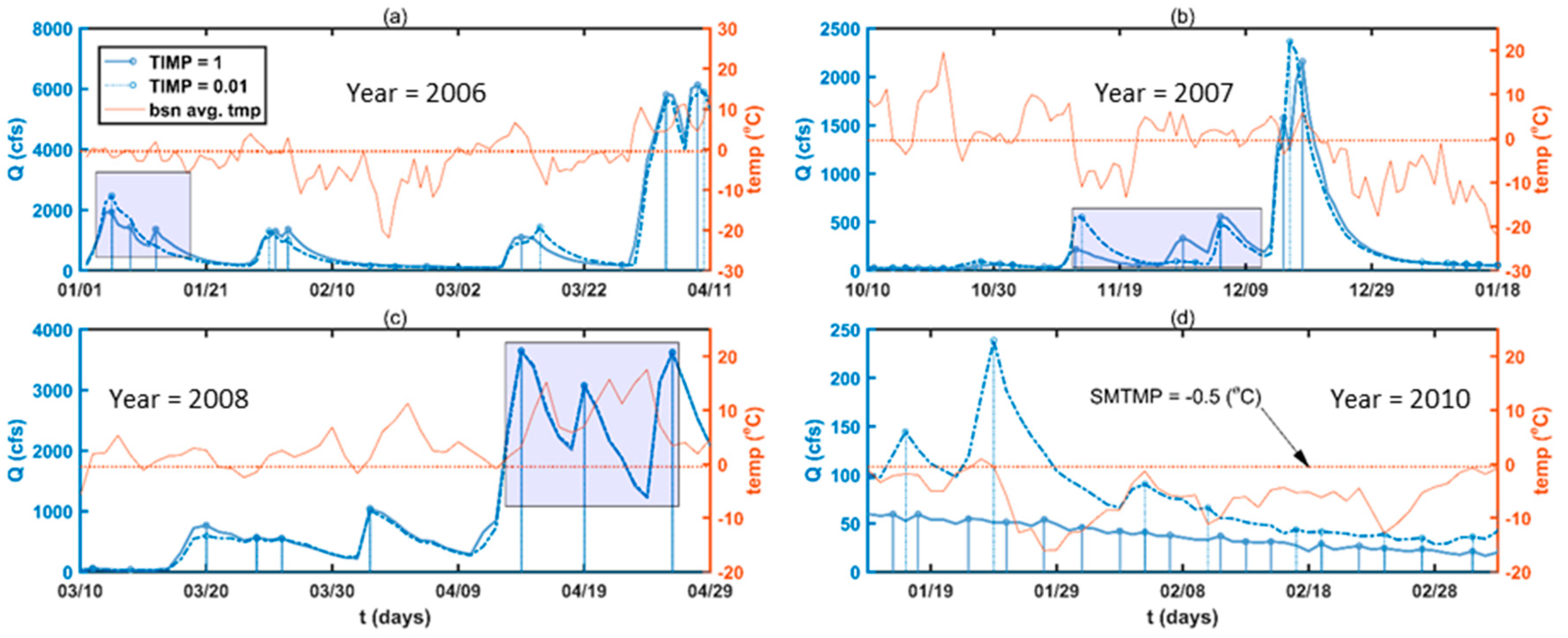
We illustrate challenges in linking parameters and streamflow outcomes using a basin level SWAT parameter TIMP and the threshold temperature for snowmelt, referred to as SMTMP. Both these parameters are pure calibration parameters [61] and are discussed as such in this paper. Several SWAT parameters are specified at the spatial resolution of the basin in this study, e.g., TIMP and SMTMP. We specify these two parameters at the basin scale due to the relatively flat topography and lack of data at a more detailed scale. Adjustment of these parameters will have basin-wide implications. A higher TIMP value (max = 1) indicates a strong influence of current day temperature on the temperature of the snow pack and a low TIMP value (min = 0.01) indicates a greater influence of the previous day’s temperature. SMTMP (°C) is defined as base temperature at which snow is allowed to melt in SWAT [55]. One way to select parameters is by identifying factors and periods when they will have an effect. By comparing with a measured parameter like air temperature, we can identify candidates for calibration provided they are sensitive for the time period of interest. This approach goes beyond a blanket sensitivity analysis, which does not consider physics associated with the parameter.
Changes in streamflow at MN 66 gage (gage 8 in Figure 1) from the LSRB model is used to illustrate analysis in the time domain. The blue box in Figure 3a,b highlights time periods (years 2006 and 2007, respectively), where significant offsets between streamflow for the scenario with TIMP = 1 and TIMP = 0.01 can be observed. Results demonstrate that TIMP is sensitive when the air temperature persists in sub-zero temperatures. The sensitivity is most clearly seen in the year 2010, when temperatures persisted below zero for nearly a month and a half (Figure 3d). When temperature rises above zero, the parameter has no effect in the outcome as can be seen for the year 2008 (See Figure 3c blue box). Multiple years are shown instead of just one to illustrate that the behavior is not a random occurrence. Scrutinizing the effects of TIMP in this way allows us to better understand its influence on the magnitude, as well as the timing of streamflow.
3.5.2. Parameter Behavior in the Frequency Domain (via Wavelet Analysis)
Time domain analysis, such as that presented in Section 3.5.1, allows us to see changes in streamflow response when a parameter is adjusted visually. Frequency domain analysis is a complementary approach to evaluate the effects of parameter adjustment. Analyzing the frequency content of a signal using wavelets can provide the frequency content that is localized in time [62]. The wavelet approach offers a targeted form of sensitivity analysis compared to the blanket approach using only lumped metrics.
The wavelet transform is an integral transform that allows for the evaluation of the temporal evolution of frequency content contained in a nonstationary signal [63,64] such as streamflow. Wavelets are functions that have a specified window where they are non-zero. These functions can be dilated or stretched to check the presence of a particular frequency in the signal. In wavelet analysis, lower scales correspond to higher frequencies and vice versa. The resulting wavelet coefficients represent the correlation between the signal at different points along the signal and at multiple scales [65]. At any scale along the vertical axis and at any point representing time along the horizontal axis, larger coefficients are indicative of greater correspondence between the analyzing wavelet and the analyzed signal (e.g., streamflow). Each scale corresponds to the width of the wavelet or the length of the signal that will be analyzed.
Following a wavelet transform, comparison in the frequency domain can be thought of as a way to compare the constituent shapes (individual frequencies) present in each signal. The coefficients that result from each signal can be compared to each other via wavelet coherence, which is analogous to R2 in statistics [66]. A coefficient value close to one indicates the frequency/shape is present in both signals for the time period under consideration. Wavelet coherence analysis of the pre-parameter adjustment signal and the post-parameter adjustment signal allows us to identify specific scales and time periods when parameter adjustments will impact the signal of interest (here, streamflow).
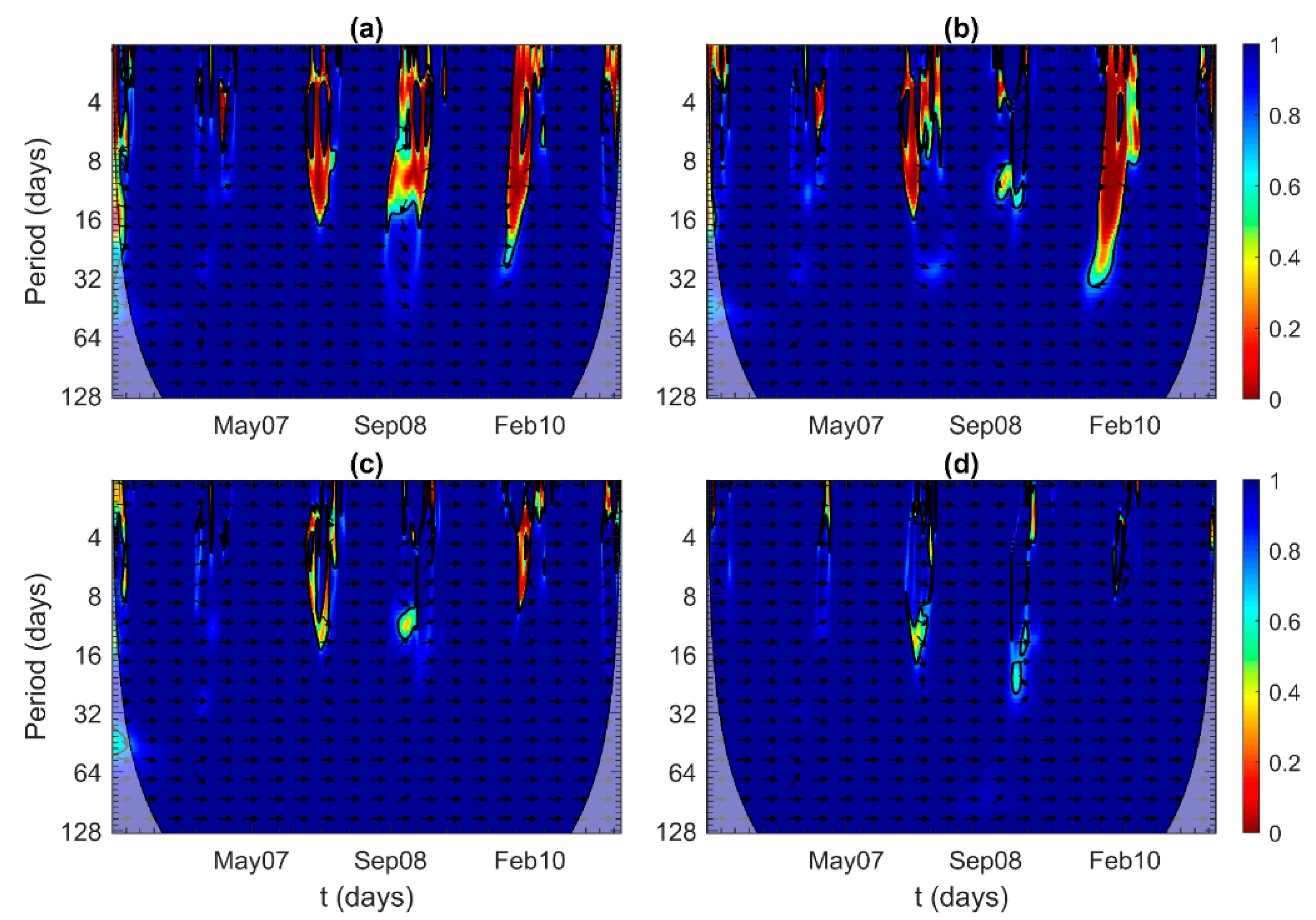
Figure 4a–d shows wavelet coherence between pre- and post-adjustment signals for four pure calibration parameters. Hotter colors (red) indicate the shape is absent in one of the signals or is a poor match between the signals, whereas cooler colors (blue) indicate that the shapes match between the two signals. The extent (time and scale) and influence (hotter colors) of a parameter is coded in color. We can see the scales and time periods where the parameters are sensitive. For example, TIMP (See Figure 4a) is only sensitive up to approximately the 32-day band and between November and March. Therefore, if there are mismatches between measured and simulated flow outside this time period or beyond a 32-day band, TIMP cannot resolve the mismatch. Similarly, for snowfall temperature (°C) (SFTMP), melt factor for snow on 21 June (mm H2O/°C-day) (SMFMX) and melt factor for snow on 21 December (mm H2O/°C-day) (SMFMN) and frozen soil infiltration factor (CN_FROZ), shown in Figure 4b–d, adjustment only affects some portions of the signal and some scales. In this case, a mismatch between the signals for any time periods other than where hotter colors are observed would essentially constitute a tuning for the wrong reason. A brief description of the parameters used to illustrate parameter selection using wavelet analysis are provide in Table S1. In Figure 4d, the time periods where there are mismatches are not continuous, indicating selective bands of influence or sensitivity. The tools developed to conduct this analysis are distributed as part of the HydroME Toolbox.
4. Meaningful Measures for Evaluating Model Performance
Models can be developed for a variety of applications and the metrics used to evaluate them should be targeted to the application of interest. For example, it is generally recognized that a good agreement between modeled and measured streamflow should involve: (1) shape of the hydrograph, (2) the timing, rate and the volume of peak flows, and (3) low flows as described in [23]. Others have reported five hydrologic metrics that are relevant for ecology and water quality, including (1) magnitude, (2) frequency, (3) duration, (4) timing and (5) rate of hydrograph rise and fall [30,67,68,69]. Yet, in practice, metrics used to evaluate their performance are commonly limited to visual inspection [70], RMSE, R2 or NSE. Better-targeted model performance metrics facilitate more efficient and robust calibration and will help the modeler make a more compelling case that the model is suitable for the application of interest.
In the following paragraphs, we introduce a simple variation in how common classical error measures are reported and show that by combining them with other graphical representations to evaluate model performance they can serve as a powerful model evaluation tool. The HydroME Toolbox that generates the graphs and performance metrics described below can be downloaded for free from: https://qcnr.usu.edu/labs/belmont_lab/resources.
Automated and intervention type calibration in hydrology generally rely on a lumped model performance metric such as NSE (a normalized measure ranging between −inf to 1.0) or R2 [27,71]. Such metrics are useful insofar as they are objective measures that can be used to quantify model behavior and can be readily and quantitatively compared among models [27]. Studies have highlighted the need for other measures in a multi-objective criteria approach for a robust evaluation of model performance [5,72]. The use of a single measure serves well in an automatic calibration context, but does not necessarily capture the most relevant aspects of model performance [71]. For example, the quadratic formulation of NSE or R2 emphasizes higher magnitude flows, relative to lower flows, the latter of which may be critical for many ecological and water quality applications [26]. Furthermore, the character of a watershed and the time step of evaluation have been shown to influence evaluation metrics and could potentially place false confidence in the ability of a hydrologic model to simulate streamflow [27,28,37]. These variance-based lumped error measures also do not separate different flow components or time dependencies [67].
We advocate for the continued use of lumped model performance metrics as they serve a useful purpose to determine offsets in flow magnitude (Table 1). Nevertheless, given the current level of sophistication of hydrologic modeling and increasing demand for models that target specific hydrologic metrics (e.g., summer base flows, timing and rate of the rising limb of the snowmelt hydrograph), other metrics such as presented here can provide valuable, additional perspective of the same data.
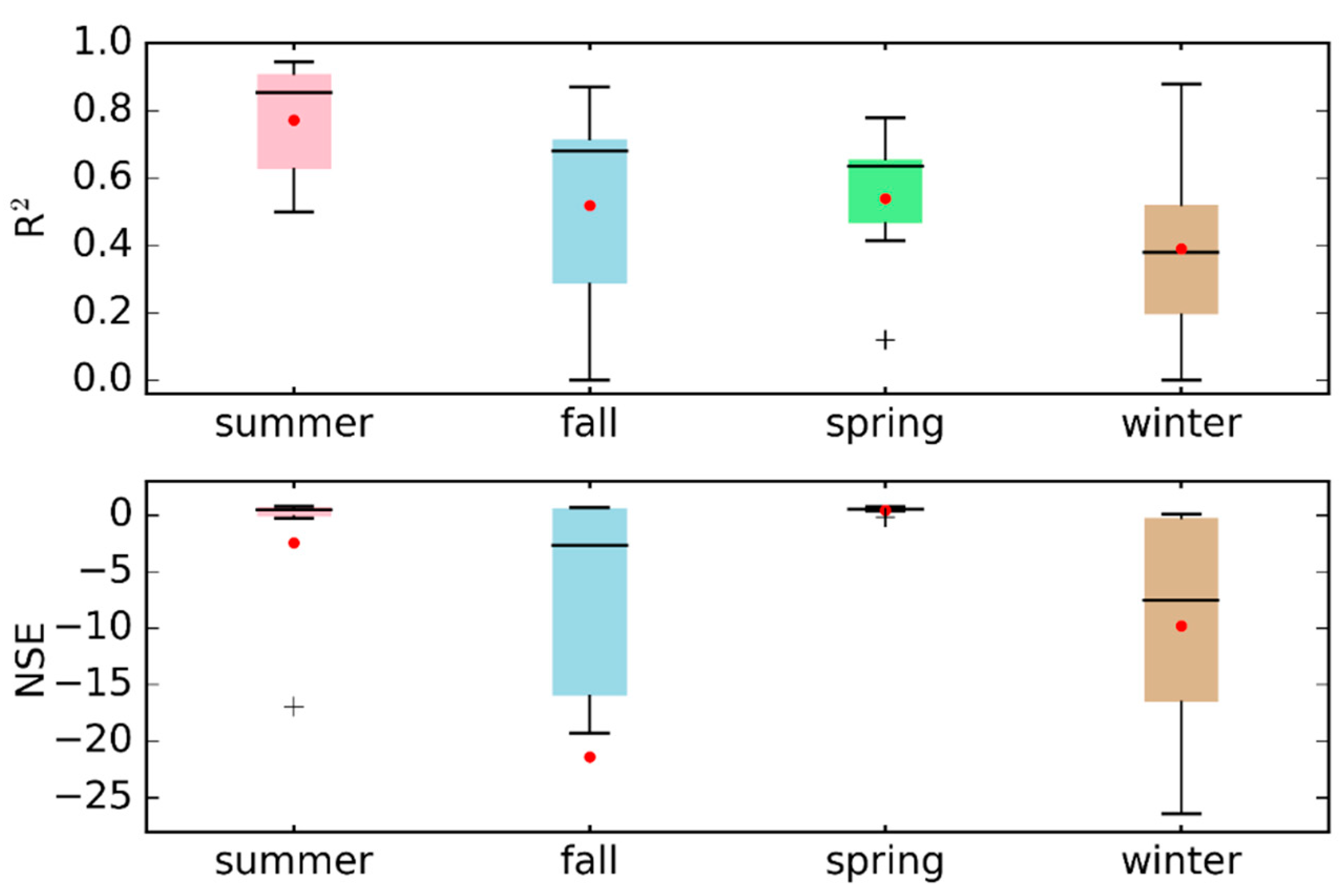
Windowing the signal into different time periods (seasons, months, etc.) can provide useful information regarding model performance. Here we propose to go a step further and use box plots to report performance measures such as NSE and R2 by aggregating them into annual, seasonal or monthly intervals as shown in Figure 5. The advantage of such a representation is that these plots can clearly show the range and distribution of the performance metric as opposed to just a central tendency value. Generally, the mean of a performance metric is reported, but that approach may obscure how well the model is performing for the time period of interest. For example, Figure 5 shows that model performance varies considerably during the fall and winter months and is captured by both metrics; NSE and R2. Both metrics are shown for the calibrated model of the RRB SWAT model. We wanted to illustrate that when we use the entire flow record for the time period when the model was calibrated, the NSE and R2 values are 0.69 and 0.70 respectively. However, when we take this same data and segregate them into seasons we see a different, and far more complete, picture. Therefore, if a modeler is interested in a particular season, it may be critical to verify model performance for the season or period of interest. Additional useful information is the Interquartile Range (IQR), which is lowest for spring irrespective of the metric considered and shows clustering around the central tendency. Additionally, the negative skew shows that most of the time the model performance is not as good as what is represented by just the central tendency. The HydroME toolbox generates the seasonal NSE and R2 plots. Additionally, the tool also generates Euclidean distance, empirical Q-Q and FDCs and is described in Section S6 of the SI .
5. Reporting: Model Performance Metrics
In addition to the time domain metric described in the previous section, frequency domain analysis can provide useful insights for model evaluation. Watershed behavior is complex and representing the data in both time and frequency domains can allow us to glean information that may be obscured when examined solely in either domain. Although these approaches can further constrain inaccurate representations of the physical system, calibration should not be substituted for best available data as no amount of forcing can achieve calibration if the model structure is inappropriate or the data are of poor quality [4]. In this section, we introduce two frequency domain methods that evaluate the shape of the hydrograph; namely, magnitude squared coherence and wavelet coherence.
5.1. Model Evaluation Using Magnitude Squared Coherence
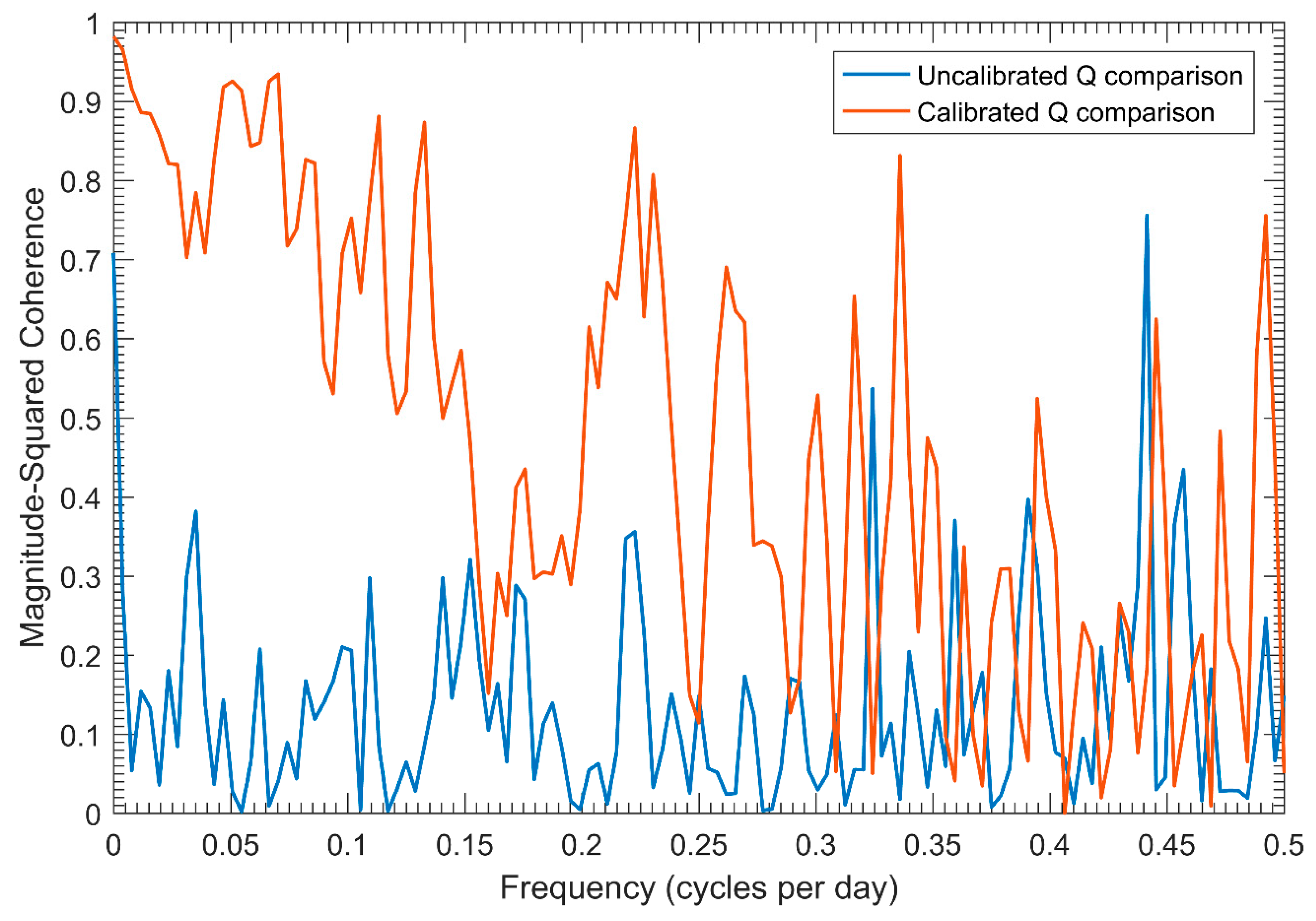
We can evaluate the performance of a model by determining if the frequency components of the measured signal are present in the simulated signal. The magnitude squared coherence approach is used to compare the frequency content of measured and simulated signals and provides a measure of their similarity [73]. The technique captures all the frequencies present in the analyzed signal without localizing the frequency. The coherence estimate provides a general sense of model performance and can reveal which flow frequencies in the measured signal were captured by the model. The specific coherence technique used here is called the magnitude squared coherence via weighted overlapped segment averaging. It measures the strength of association between two stationary stochastic processes [74]. With the assumption of a stationary stochastic process, we ignore the time at which the frequency occurred in the signal. We acknowledge that such an assumption could result in a false positive (i.e., a given frequency could be present in both signals, but occur at different times); however, this issue can be resolved with the wavelet analysis, which has a different set of advantages and limitations, as discussed in Section 5.2. When the processes that determine the flow outcome are independent or absent, a coherence of zero should be expected and a value of one when they are dependent or present. Prior to calibration, most frequencies that characterize the observed streamflow are absent in the uncalibrated model-predicted signal (Figure 6). After calibration, the frequency spectra of observed flows and model predictions are far more similar. For example, note the higher coherence values across the spectrum and especially for frequencies below 0.25 (wavelength of 4 days) in Figure 6). It can be seen even with calibration; some frequencies are absent in the simulated signal. The magnitude-squared coherence, is defined as shown in Equation (1),
where, is a complex cross spectral density, and are auto spectral densities at a particular frequency f [74].
5.2. Wavelet Coherence for Model Performance Evaluation
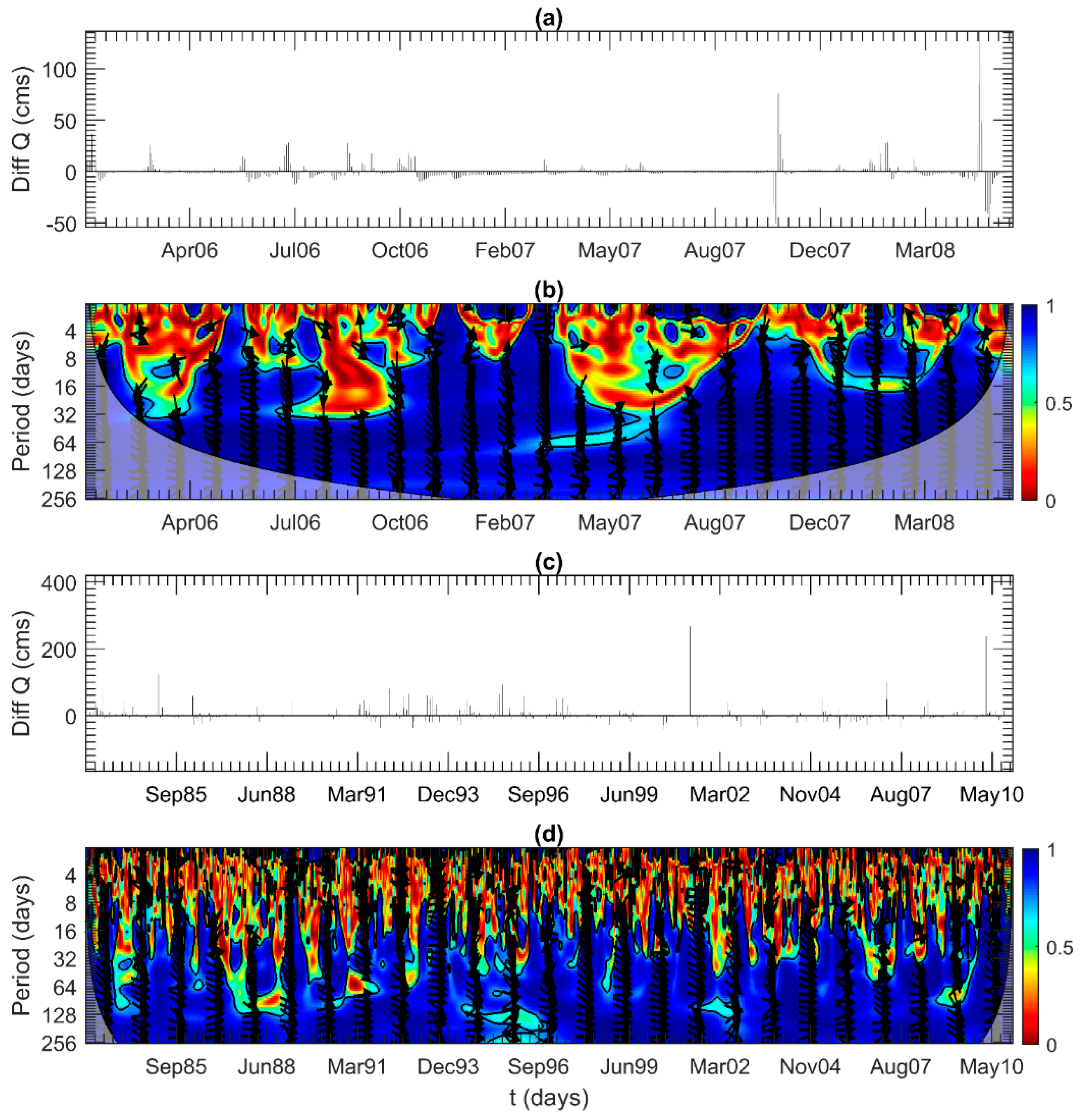
Comparing model performance using the magnitude squared coherence approach compares all frequencies present in the signal; however, it cannot localize the mismatch in time. This results in the loss of time information [75]. Moreover, the global nature of lumped error metrics (e.g., NSE, R2) is of little use when event scale predictions or time resolution of model performance is needed. Instead, coherence calculated using wavelets can provide this information. Specifically, the time-frequency representation of measured and simulated signals allows us to clearly see (1) if there are any patterns in the model’s inability to simulate observed flows, and (2) the times and frequencies for which the model was able to capture the measured streamflow. In Figure 7a,c, the residuals show the time periods when there are differences between the measured and predicted streamflow. This time domain view provides insights into the time and magnitude of discrepancies. In Figure 7b, the wavelet coherence plot shows that frequencies below the 32-day band are generally not captured well, except for a few locations. Beyond the 32-day band, we see a nearly 100% capture of the measured signal by the model. In Figure 7d, we see mismatches up to the 128-day band during certain time periods. However, there are time periods when the higher frequencies are captured well by the model.
6. Discussion and Conclusions
Watershed hydrology models have advanced considerably over the past decade. With increasing capabilities and demands on such models, it is essential that the hydrologic community embrace more targeted and meaningful metrics for model evaluation. In this paper, we have introduced and tested a suite of new tools for model evaluation, suggest a hierarchical approach to the selection of parameters to adjust during calibration, and discuss the benefits of evaluating models in both time and frequency domains. Methods described in this paper were applied to two model instances representing physical environments that challenge calibration in different ways.
Starting with an appropriate model structure and high-quality input data are essential for developing a useful and reliable model. Generally speaking, more and diverse types of observations is the primary approach to constrain or reduce equifinality. However, in most cases, data is still limited to streamflow and available only at few gages with short time periods. Therefore, we need other ways to address the challenge. Here, we describe an approach where we show by not including certain parameters from calibration, the number of combinations we have is reduced (i.e., constraining equifinality). Excluding certain parameters recognizes that some parameters have a more robust scientific basis than others, in their initialized values.
Most hydrology models require some form of calibration as many of the parameters are only conceptual and cannot be measured in the field. Even parameters that can be measured in the field may not always be available or present at the spatial resolution needed. Thus, a hierarchical approach to parameter adjustment, starting with the most uncertain parameters, is recommended. We show equifinality and interdependencies among parameters present formidable challenges for fully automated calibration procedures. For example, automated routines depend on lumped metrics and cannot uniquely identify parameter sets that optimize calibration while minimizing distortion of the physical system, even with the use of multi-objective lumped metrics. Many parameter combinations, representing different characterizations of the physical system, result in local maxima for numerous evaluation criteria. Further, there are pitfalls of using a blanket sensitivity-based approach in the selection of parameters to adjust for calibration, which has the potential to render a model unable to reliably simulate certain management practices. Reliance on the Curve Number method widely within the SWAT framework to inform management decisions for implementing various conservation practices must be implemented with caution.
We illustrate that choosing parameters through both time and frequency domains provides complementary strengths that can be leveraged to identify parameters for calibration. Scenarios can be evaluated by comparing different values of the same parameter along with related observations to identify time periods and magnitudes of mismatch. Frequency domain analysis can provide insight in cases when there are complex interactions between parameters as physics-based explanations for parameter adjustments may be inadequate. Wavelet transform provides the description of frequencies in a hydrologic signal that are localized by time. The magnitude squared coherence and wavelet analyses are most useful in the latter stages of calibration and model evaluation, after major parameter adjustments have been made based on lumped metrics and other time domain metrics.
We provide a guideline for prioritizing parameters during calibration based on the information we have about the particular parameter. The primary motivation for such a classification is to minimize physical distortion through parameter adjustment. In this paper, we classify parameters into three categories, namely; pure, derived and measured based on the amount of uncertainty. We also demonstrate the flexible nature of the classification as the amount information known for any particular parameter can vary with study area or access to information. Modifying model structure may also be necessary to achieve adequate model calibration. However, we encourage using a model structure that is appropriate for time scales of evaluation, the questions of interest, and the environment under consideration.
Lumped metrics make it easy to evaluate model performance with one all-inclusive value. However, reporting lumped metrics by segregating them annually or monthly using box-plots can reveal considerable information about model performance that are otherwise obscured by the central tendency-based approach. Euclidian distance measures can be used to identify magnitude mismatches that are localized in time. Empirical Q-Q plots show the quantiles that were captured by the model and aid in calibration. FDCs can be another technique that can reveal what the model is able to simulate. Further exploration is needed for specifically identifying parameters that can help remove any mismatch.
We have demonstrated the value of frequency and time-frequency domain measures to report model performance. Magnitude squared coherence was used to compare the measured and predicted signals, which highlighted that even for a NSE value of 0.74 many of the frequencies were missing in the predicted flow. This approach, however, did not resolve the time of mismatch. The use of wavelet coherence allowed for a time resolution of frequency comparison. The measured and simulated flows showed a general mismatch in the higher frequencies which were delineated both by time and scale. Like lumped metrics or other time domain model performance measures, we cannot fully and unambiguously separate the sources of mismatch, which could be attributed to data, model structure or the calibration itself. In that context, it is useful to reiterate that models are developed for a variety of applications and the metrics used to evaluate them should be targeted to the application of interest.
Supplementary Materials
The following are available online at https://www.mdpi.com/2073-4441/10/6/710/s1, Sections S1 to S7, Figures S1 to S8, and Tables S1 to S5.
Author Contributions
K.K. developed the methodology, obtained and analyzed the data, and wrote the initial draft. P.B. contributed to development of the ideas, interpretation of results and writing of the manuscript.
Acknowledgments
This work was made possible with support from the National Science Foundation (NSF ENG 1209445), US Department of Agriculture NRCS (69-3A75-14-269), and the Utah State University Agricultural Experiment Station, approved as paper #9104. A preliminary version of this study can be found at https://www.hydrol-earth-syst-sci-discuss.net/hess-2017-121/. We thank the anonymous reviewers and the Editor for their suggestions which has substantially improved the manuscript.
Conflicts of Interest
The authors declare no conflict of interest.
References
- Santhi, C.; Arnold, J.G.; White, M.; Di Luzio, M.; Kannan, N.; Norfleet, L.; Atwood, J.; Kellogg, R.; Wang, X.; Williams, J.R.; et al. Effects of agricultural conservation practices on N loads in the Mississippi-Atchafalaya River basin. J. Environ. Qual. 2014, 43, 1903–1915. [Google Scholar] [CrossRef] [PubMed]
- Kouchi, D.H.; Esmaili, K.; Faridhosseini, A.; Sanaeinejad, S.H.; Khalili, D.; Abbaspour, K.C. Sensitivity of calibrated parameters and water resource estimates on different objective functions and optimization algorithms. Water 2017, 9, 384. [Google Scholar] [CrossRef]
- Kamali, B.; Abbaspour, K.; Yang, H. Assessing the uncertainty of multiple input datasets in the prediction of water resource components. Water 2017, 9, 709. [Google Scholar] [CrossRef]
- Abbaspour, K.; Vaghefi, S.; Srinivasan, R. A guideline for successful calibration and uncertainty analysis for Soil and Water Assessment: A review of papers from the 2016 International SWAT Conference. Water 2018, 10, 6. [Google Scholar] [CrossRef]
- Singh, V.P.; Frevert, D.K. Mathematical Models of Large Watershed Hydrology; Water Resources Publication: Littleton, CO, USA, 2002. [Google Scholar]
- Beven, K.J. Rainfall-Runoff Modelling: The Primer; John Wiley & Sons: Hoboken, NJ, USA, 2011. [Google Scholar]
- Sorooshian, S.; Gupta, V.K. Automatic calibration of conceptual rainfall-runoff models: The question of parameter observability and uniqueness. Water Resour. Res. 1983, 19, 260–268. [Google Scholar] [CrossRef]
- Beven, K. A manifesto for the equifinality thesis. J. Hydrol. 2006, 320, 18–36. [Google Scholar] [CrossRef] [Green Version]
- Madsen, H. Parameter estimation in distributed hydrological catchment modelling using automatic calibration with multiple objectives. Adv. Water Resour. 2003, 26, 205–216. [Google Scholar] [CrossRef]
- Beven, K.; Freer, J. Equifinality, data assimilation, and uncertainty estimation in mechanistic modelling of complex environmental systems using the glue methodology. J. Hydrol. 2001, 249, 11–29. [Google Scholar] [CrossRef]
- Gupta, H.V.; Sorooshian, S.; Yapo, P.O. Toward improved calibration of hydrologic models: Multiple and noncommensurable measures of information. Water Resour. Res. 1998, 34, 751–763. [Google Scholar] [CrossRef]
- Faramarzi, M.; Srinivasan, R.; Iravani, M.; Bladon, K.D.; Abbaspour, K.C.; Zehnder, A.J.B.; Goss, G.G. Setting up a hydrological model of Alberta: Data discrimination analyses prior to calibration. Environ. Model. Softw. 2015, 74, 48–65. [Google Scholar] [CrossRef]
- Taddele, D.Y.; Raghavan, S. Evaluation of CFSR climate data for hydrologic prediction in data-scarce watersheds: An application in the Blue Nile River basin. JAWRA J. Am. Water Resour. Assoc. 2014, 50, 1226–1241. [Google Scholar]
- Zambrano-Bigiarini, M. HydroGOF: Goodness-of-fit functions for comparison of simulated and observed hydrological time series. R package version 0.3-8. Available online: http://hzambran.github.io/hydroGOF/ (accessed on 12 October 2017).
- Dawson, C.W.; Abrahart, R.J.; See, L.M. Hydrotest: A web-based toolbox of evaluation metrics for the standardised assessment of hydrological forecasts. Environ. Model. Softw. 2007, 22, 1034–1052. [Google Scholar] [CrossRef]
- Ritter, A.; Muñoz-Carpena, R. Performance evaluation of hydrological models: Statistical significance for reducing subjectivity in goodness-of-fit assessments. J. Hydrol. 2013, 480, 33–45. [Google Scholar] [CrossRef]
- Willems, P.; Mora, D.; Vansteenkiste, T.; Taye, M.T.; Van Steenbergen, N. Parsimonious rainfall-runoff model construction supported by time series processing and validation of hydrological extremes—Part 2: Intercomparison of models and calibration approaches. J. Hydrol. 2014, 510, 591–609. [Google Scholar] [CrossRef]
- Willems, P. Parsimonious rainfall-runoff model construction supported by time series processing and validation of hydrological extremes—Part 1: Step-wise model-structure identification and calibration approach. J. Hydrol. 2014, 510, 578–590. [Google Scholar] [CrossRef]
- Willems, P. A time series tool to support the multi-criteria performance evaluation of rainfall-runoff models. Environ. Model. Softw. 2009, 24, 311–321. [Google Scholar] [CrossRef]
- Chen, J.; Wu, Y. Advancing representation of hydrologic processes in the Soil and Water Assessment Tool (SWAT) through integration of the TOPographic model (TOPMODEL) features. J. Hydrol. 2012, 420–421, 319–328. [Google Scholar] [CrossRef]
- Weiler, M.; Beven, K. Do we need a community hydrological model? Water Resour. Res. 2015, 51, 7777–7784. [Google Scholar] [CrossRef]
- Centre for Agriculture and Rural Development (CARD). ISU of Science and Technology. SWAT Literature Database for Peer-Reviewed Journal Articles. Available online: https://www.card.iastate.edu/swat_articles/ (accessed on 12 December 2016).
- Madsen, H. Automatic calibration of a conceptual rainfall–runoff model using multiple objectives. J. Hydrol. 2000, 235, 276–288. [Google Scholar] [CrossRef]
- Douglas-Mankin, K.R.; Srinivasan, R.; Arnold, J.G. Soil and Water Assessment Tool (SWAT) model: Current developments and applications. Trans. ASABE 2010, 53, 1423–1431. [Google Scholar] [CrossRef]
- Moriasi, D.N.; Gitau, M.W.; Pai, N.; Daggupati, P. Hydrologic and water quality models: Performance measures and evaluation criteria. Trans. ASABE 2015, 58, 1763–1785. [Google Scholar]
- Criss, R.E.; Winston, W.E. Do Nash values have value? Discussion and alternate proposals. Hydrol. Process. 2008, 22, 2723–2725. [Google Scholar] [CrossRef]
- Krause, P.; Boyle, D.P.; Bäse, F. Comparison of different efficiency criteria for hydrological model assessment. Adv. Geosci. 2005, 5, 89–97. [Google Scholar] [CrossRef]
- Schaefli, B.; Gupta, H.V. Do Nash values have value? Hydrol. Process. 2007, 21, 2075–2080. [Google Scholar] [CrossRef]
- Gupta, H.V.; Kling, H.; Yilmaz, K.K.; Martinez, G.F. Decomposition of the mean squared error and NSE performance criteria: Implications for improving hydrological modelling. J. Hydrol. 2009, 377, 80–91. [Google Scholar] [CrossRef]
- Lytle, D.A.; Poff, N.L. Adaptation to natural flow regimes. Trends Ecol. Evol. 2004, 19, 94–100. [Google Scholar] [CrossRef] [PubMed]
- Sanborn, S.C.; Bledsoe, B.P. Predicting streamflow regime metrics for ungauged streams in Colorado, Washington, and Oregon. J. Hydrol. 2006, 325, 241–261. [Google Scholar] [CrossRef]
- Wenger, S.J.; Luce, C.H.; Hamlet, A.F.; Isaak, D.J.; Neville, H.M. Macroscale hydrologic modeling of ecologically relevant flow metrics. Water Resour. Res. 2010, 46. [Google Scholar] [CrossRef]
- Wilcock, P.R.; Belmont, P. Identifying Sediment Sources in the Minnesota River Basin; Public Synthesis Report for the Minnesota River Sediment Colloquium; Minnesota Pollution Control Agency: St. Paul, MN, USA, 2009.
- Belmont, P.; Gran, K.B.; Schottler, S.P.; Wilcock, P.R.; Day, S.S.; Jennings, C.; Lauer, J.W.; Viparelli, E.; Willenbring, J.K.; Engstrom, D.R.; et al. Large shift in source of fine sediment in the Upper Mississippi river. ESandT 2011, 45, 8804–8810. [Google Scholar] [CrossRef] [PubMed]
- Minnesota State University, Mankato Water Resources Center (MSU-WRC); Minnesota Pollution Control Agency (MPCA). State of the Minnesota River: Summary of Surface Water Quality Monitoring 2000–2008; Minnesota River Basin Data Center: Mankato, MN, USA, 2009; p. 42.
- Belmont, P.; Willenbring, J.K.; Schottler, S.P.; Marquard, J.; Kumarasamy, K.; Hemmis, J.M. Toward generalizable sediment fingerprinting with tracers that are conservative and nonconservative over sediment routing timescales. J. Soils Sediments 2014, 14, 1479–1492. [Google Scholar] [CrossRef]
- Belmont, P.; Stevens, J.R.; Czuba, J.A.; Kumarasamy, K.; Kelly, S.A. Comment on “climate and agricultural land use change impacts on streamflow in the upper midwestern united states,” by Satish C. Gupta et al. Water Resour. Res. 2016, 52, 7523–7528. [Google Scholar] [CrossRef]
- U.S. Geological Survey (USGS). USGS NED n44w093 1/3 Arc-Second 2013 1 x 1 Degree ArcGrid; USGS: Reston, VA, USA, 2013.
- U.S. Geological Survey (USGS). USGS NED n44w092 1/3 Arc-Second 2013 1 x 1 Degree ArcGrid; USGS: Reston, VA, USA, 2013.
- Han, W.-G.; Yang, Z.-W.; Di, L.-P.; Yue, P. A geospatial web service approach for creating on-demand cropland data layer thematic maps. Trans. ASABE 2014, 57, 239–247. [Google Scholar]
- Soil Survey Staff. Soil Survey Geographic (SSURGO) Database; Natural Resources Conservation Service (NRCS): Washington, DC, USA, 2015.
- PRISM Climate Group. Descriptions of PRISM Spatial Climate Datasets for the Conterminous United States; Oregon State University: Corvallis, OR, USA, 2004. [Google Scholar]
- Saha, S.; Moorthi, S.; Wu, X.; Wang, J.; Nadiga, S.; Tripp, P.; Behringer, D.; Hou, Y.-T.; Chuang, H.-Y.; Iredell, M.; et al. The NCEP climate forecast system version 2. J. Clim. 2014, 27, 2185–2208. [Google Scholar] [CrossRef]
- Arnold, J.G.; Allen, P.M.; Muttiah, R.; Bernhardt, G. Automated base flow separation and recession analysis techniques. Groundwater 1995, 33, 1010–1018. [Google Scholar] [CrossRef]
- Arnold, J.G.; Allen, P.M. Automated methods for estimating baseflow and ground water recharge from streamflow records. J. Am. Water Resour. Assoc. 1999, 35, 411–424. [Google Scholar] [CrossRef]
- Minnesota Pollution Control Agency (MPCA). Root River Watershed Monitoring and Assessment Report; MPCA: St. Paul, MN, USA, 2012.
- Baffaut, C.; Benson, V.W. Modeling flow and pollutant transport in a karst watershed with SWAT. Trans. ASABE 2009, 52, 469–479. [Google Scholar] [CrossRef]
- Belmont, P.; Dogwiler, T.; Kumarasamy, K. An Integrated Sediment Budget for the Root River Watershed, Southeastern Minnesota; Final Report; Minnesota Department of Agriculture: St. Paul, MN, USA, 2016. [Google Scholar]
- Madsen, H.; Wilson, G.; Ammentorp, H.C. Comparison of different automated strategies for calibration of rainfall-runoff models. J. Hydrol. 2002, 261, 48–59. [Google Scholar] [CrossRef]
- Tolson, B.A.; Shoemaker, C.A. Dynamically dimensioned search algorithm for computationally efficient watershed model calibration. Water Resour. Res. 2007, 43. [Google Scholar] [CrossRef]
- Efstratiadis, A.; Koutsoyiannis, D. One decade of multi-objective calibration approaches in hydrological modelling: A review. Hydrol. Sci. J. 2010, 55, 58–78. [Google Scholar] [CrossRef]
- Fatichi, S.; Vivoni, E.R.; Ogden, F.L.; Ivanov, V.Y.; Mirus, B.; Gochis, D.; Downer, C.W.; Camporese, M.; Davison, J.H.; Ebel, B.; et al. An overview of current applications, challenges, and future trends in distributed process-based models in hydrology. J. Hydrol. 2016, 537, 45–60. [Google Scholar] [CrossRef]
- Hill, M.C. Methods and Guidelines for Effective Model Calibration; With Application to UCODE, a Computer Code for Universal Inverse Modeling, and MODFLOWP, a Computer Code for Inverse Modeling with MODFLOW; Water-Resources Investigations Report 98-4005; U.S. Geological Survey, Branch of Information Services: Reston, VA, USA, 1998.
- Doherty, J.; Skahill, B.E. An advanced regularization methodology for use in watershed model calibration. J. Hydrol. 2006, 327, 564–577. [Google Scholar] [CrossRef]
- Arnold, J.G.; Moriasi, D.N.; Gassman, P.W.; Abbaspour, K.C.; White, M.J.; Srinivasan, R.; Santhi, C.; Harmel, R.D.; van Griensven, A.; Van Liew, M.W.; et al. SWAT: Model use, calibration, and validation. Trans. ASABE 2012, 55, 1491–1508. [Google Scholar] [CrossRef]
- Beven, K.; Binley, A. The future of distributed models: Model calibration and uncertainty prediction. Hydrol. Process. 1992, 6, 279–298. [Google Scholar] [CrossRef]
- Neitsch, S.L.; Williams, J.; Arnold, J.; Kiniry, J. Soil and Water Assessment Tool Theoretical Documentation Version 2009; Texas Water Resources Institute: College Station, TX, USA, 2011. [Google Scholar]
- Dahlke, H.E.; Easton, Z.M.; Walter, M.T.; Steenhuis, T.S. Field test of the variable source area interpretation of the curve number rainfall-runoff equation. J. Irrig. Drain. Eng. 2012, 138, 235–244. [Google Scholar] [CrossRef]
- Steenhuis, T.S.; Winchell, M.; Rossing, J.; Zollweg, J.A.; Walter, M.F. SCS runoff equation revisited for variable-source runoff areas. J. Irrig. Drain. Eng. 1995, 121, 234–238. [Google Scholar] [CrossRef]
- United States Department of Agriculture-Natural Resources Conservation Service (USDA-NRCS). Section 16: Drainage of agricultural lands. In National Engineering Handbook; USDA-NRCS: Washington, DC, USA, 1971. [Google Scholar]
- Wang, X.; Melesse, A. Evaluation of the SWAT model's snowmelt hydrology in a northwestern Minnesota watershed. Trans. ASAE 2005, 48, 1359–1376. [Google Scholar] [CrossRef]
- Paul, S.A. Wavelet transforms and the ECG: A review. Physiol. Meas. 2005, 26, R155–R199. [Google Scholar]
- Pichot, V.; Gaspoz, J.-M.; Molliex, S.; Antoniadis, A.; Busso, T.; Roche, F.; Costes, F.; Quintin, L.; Lacour, J.-R.; Barthélémy, J.-C. Wavelet transform to quantify heart rate variability and to assess its instantaneous changes. J. Appl. Physiol. 1999, 86, 1081–1091. [Google Scholar] [CrossRef] [PubMed]
- Foufoula-Georgiou, E.; Kumar, P. Wavelets in Geophysics; Academic Press: Oxford, MA, USA, 2014; Volume 4. [Google Scholar]
- Percival, D.P. On estimation of the wavelet variance. Biometrika 1995, 82, 619–631. [Google Scholar] [CrossRef]
- Liu, P.C. Wavelet spectrum analysis and ocean wind waves. In Wavelet Analysis and Its Applications; Foufoula-Georgiou, E., Kumar, P., Eds.; Academic Press: Cambridge, MA, USA, 1994; Volume 4, pp. 151–166. [Google Scholar]
- Liu, Y.; Brown, J.; Demargne, J.; Seo, D.-J. A wavelet-based approach to assessing timing errors in hydrologic predictions. J. Hydrol. 2011, 397, 210–224. [Google Scholar] [CrossRef]
- Zolezzi, G.; Bellin, A.; Bruno, M.C.; Maiolini, B.; Siviglia, A. Assessing hydrological alterations at multiple temporal scales: Adige River, Italy. Water Resour. Res. 2009, 45, W12421. [Google Scholar] [CrossRef]
- Mathews, R.; Richter, B.D. Application of the indicators of hydrologic alteration software in environmental flow setting1. J. Am. Water Resour. Assoc. 2007, 43, 1400–1413. [Google Scholar] [CrossRef]
- Hogue, T.S.; Sorooshian, S.; Gupta, H.; Holz, A.; Braatz, D. A multistep automatic calibration scheme for river forecasting models. J. Hydrometeorol. 2000, 1, 524–542. [Google Scholar] [CrossRef]
- Reusser, D.E.; Blume, T.; Schaefli, B.; Zehe, E. Analysing the temporal dynamics of model performance for hydrological models. Hydrol. Earth Syst. Sci. 2009, 13, 999–1018. [Google Scholar] [CrossRef]
- Yapo, P.O.; Gupta, H.V.; Sorooshian, S. Multi-objective global optimization for hydrologic models. J. Hydrol. 1998, 204, 83–97. [Google Scholar] [CrossRef]
- Ropella, K.M.; Sahakian, A.V.; Baerman, J.M.; Swiryn, S. The coherence spectrum. A quantitative discriminator of fibrillatory and nonfibrillatory cardiac rhythms. Circulation 1989, 80, 112–119. [Google Scholar] [CrossRef] [PubMed]
- Wang, S.-Y.; Liu, X.; Yianni, J.; Christopher Miall, R.; Aziz, T.Z.; Stein, J.F. Optimising coherence estimation to assess the functional correlation of tremor-related activity between the subthalamic nucleus and the forearm muscles. J. Neurosci. Methods 2004, 136, 197–205. [Google Scholar] [CrossRef] [PubMed]
- Si, B.C. Spatial scaling analyses of soil physical properties: A review of spectral and wavelet methods. Vadose Zone J. 2008, 7, 547–562. [Google Scholar] [CrossRef]
Figure 1.
Map of midwestern US showing the two watersheds included in this study. Land use map of Le Sueur River Basin (LSRB) and Root River Basin (RRB) are overlaid with streamflow gages where the SWAT models were calibrated and validated. Land use from the year 2006 is shown for the two basins. Corn, soybean, forest (deciduous, evergreen and mixed forests) and all else (e.g., grass/pasture, develop/open space and others) are combined as other land use.

Figure 2.
Flexible nature of parameter classification. All parameters with the extension .bsn are specified at the spatial resolution of the entire watershed, all parameters with the extension .sub or .rte are specified at the spatial resolution of the subbasin and all other parameters are specified at the resolution of the hru. All parameters were described in a distributed setting. For example, CN2 was specified for each hru based on land use, soils type and condition. The parameters are defined in Table S1 in the SI.

Figure 3.
Daily average streamflow change from pre (TIMP = 1) to post (TIMP = 0.01) adjustment contrasted with basin average daily air temperature (derived from averaging daily air temperature from 175 subbasins). The x axis shows the date in MM/DD format. Dots indicate local peak flow values identified by the peak flow selection tool available in HydroME Toolbox. Dotted line represents the threshold temperature for snowmelt. (a) shows months January to April for year 2006; (b) shows months October to January for year 2007; (c) shows months March and April for year 2008; (d) shows months January and February for year 2010.

Figure 4.
Dissimilarity in the time-scale domain between pre and post parameter adjusted streamflow signals are shown with the Wavelet Transform Coherence (WTC). The cone of influence is represented using a lighter shade (region where edge effects become dominant). The abscissa is time and the ordinate is the wavelet scale equivalent to the Fourier period. The coherence value is encoded by color. The thick black contour lines represent the 5% significance level against red noise. The phase relationship between the pre- and post-adjusted streamflow signals is indicated with arrows, with right arrows representing a in-phase relationship; left, a anti-phase relationship, down a pre-adjusted signal leading post-adjusted signal by 90° and up post-adjusted signal leading pre-adjusted signal by 90°. Phase relationship is only shown where coherence is ≥0.5. WTC for four commonly adjusted SWAT parameters to achieve calibration are shown, where (a) is TIMP, (b) is snowfall temperature (°C) (SFTMP), (c) is melt factor for snow on 21 June (mm H2O/°C-day) (SMFMX) and melt factor for snow on 21 December (mm H2O/°C-day) (SMFMN) and (d) is frozen soil infiltration factor (CN_FROZ). Change of streamflow shown in the time-scale domain resulting from one-at-a-time parameter adjustment. All four parameters are considered as pure calibration parameters in this paper.

Figure 5.
Seasonal NSE and R2 for the Root River Basin for the calibration period. Average overall NSE and R2 for the calibration period are 0.69 and 0.70, respectively. The box and whisker plot shows the eight number summary of the performance metrics. The height of the box portion is given by the interquartile range (IQR, 25th to 75th percentile) of the performance metrics NSE and R2. The horizontal bar is the median, red dot is the mean and the whiskers represent the 10th and 90th percentile values. The extreme values are shown with a “+”.

Figure 6.
Magnitude squared coherence via Welch comparing measured streamflow with uncalibrated and calibrated streamflow. A value of 1 indicates the frequency is present in both the measured and predicted signals and a zero means it was present in one and not the other.
Figure 6.
Magnitude squared coherence via Welch comparing measured streamflow with uncalibrated and calibrated streamflow. A value of 1 indicates the frequency is present in both the measured and predicted signals and a zero means it was present in one and not the other.

Figure 7.
(a,c) Euclidian metric (between measured vs. simulated) for the Le Sueur River at St. Clair gage and Le Sueur River near Rapidan, MN 66 gage in the Le Sueur River Basin (LSRB) respectively. (b,d) Dissimilarity in time-scale domain between the measured and predicted signals are illustrated with the Wavelet Transform Coherence (WTC) for the Le Sueur River at St. Clair gage and Le Sueur River near Rapidan, MN 66 gage in LSRB respectively. The cone of influence is represented using a lighter shade (region where edge effects become dominant). The abscissa is time and the ordinate is the wavelet scale equivalent to the Fourier period. The coherence value is encoded by color. The low coherence in the ~<16 days period band is attributable to the inability of the model to capture higher frequency peak flows.


Table 1.
Lumped metrics (NSE and R2) shown as commonly reported in the literature based on separation of data into calibration and validation data sets for RRB and LSRB at daily time step.
Table 1.
Lumped metrics (NSE and R2) shown as commonly reported in the literature based on separation of data into calibration and validation data sets for RRB and LSRB at daily time step.
| Gage | Cal. | Val. | Cal. | Val. | Cal. | Val. | |
|---|---|---|---|---|---|---|---|
| NSE | R2 | PBIAS | |||||
| Root River Basin | Middle Branch | 0.60 | 0.56 | 0.70 | 0.73 | 31.41 | −49.07 |
| Houston | 0.54 | 0.59 | 0.57 | 0.61 | −3.24 | −14.78 | |
| Mound Prairie | 0.68 | 0.52 | 0.72 | 0.61 | −16.44 | −25.10 | |
| Pilot Mound | 0.69 | 0.64 | 0.70 | 0.67 | −5.72 | −16.64 | |
| South Branch | 0.50 | 0.56 | 0.67 | 0.63 | −2.78 | 13.87 | |
| Le Sueur River Basin | Le Sueur River at St. Clair, CSAH28 | 0.67 | 0.72 | 0.67 | 0.74 | 0.25 | 7.44 |
| Le Sueur River at Rapidan, CR8 | 0.57 | 0.75 | 0.57 | 0.76 | −1.97 | 1.40 | |
| LSR near Rapidan, MN66 | 0.59 | 0.73 | 0.60 | 0.74 | 15.32 | 7.67 | |
| Little Beauford Ditch | 0.54 | 0.50 | 0.55 | 0.62 | 17.72 | −23.69 | |
| Little Cobb River near Beauford | 0.74 | 0.79 | 0.76 | 0.79 | 9.90 | −2.55 | |
| Big Cobb River near Beauford, CR16 | 0.83 | 0.84 | 0.84 | 0.85 | 3.90 | 5.03 | |
| Maple River near Rapidan, CR35 | 0.72 | 0.69 | 0.73 | 0.70 | −21.66 | 7.85 | |
| Maple River near Sterling Center, CR18 | 0.72 | 0.73 | 0.70 | 0.75 | 8.76 | 17.70 | |
Note: Cal. And Val. represents calibration and validation periods respectively.
© 2018 by the authors. Licensee MDPI, Basel, Switzerland. This article is an open access article distributed under the terms and conditions of the Creative Commons Attribution (CC BY) license (http://creativecommons.org/licenses/by/4.0/).
Share and Cite
MDPI and ACS Style
Kumarasamy, K.; Belmont, P. Calibration Parameter Selection and Watershed Hydrology Model Evaluation in Time and Frequency Domains. Water 2018, 10, 710. https://doi.org/10.3390/w10060710
AMA Style
Kumarasamy K, Belmont P. Calibration Parameter Selection and Watershed Hydrology Model Evaluation in Time and Frequency Domains. Water. 2018; 10(6):710. https://doi.org/10.3390/w10060710
Chicago/Turabian StyleKumarasamy, Karthik, and Patrick Belmont. 2018. "Calibration Parameter Selection and Watershed Hydrology Model Evaluation in Time and Frequency Domains" Water 10, no. 6: 710. https://doi.org/10.3390/w10060710
Note that from the first issue of 2016, this journal uses article numbers instead of page numbers. See further details here.