Assessment of Rainfall Variability and Its Relationship to ENSO in a Sub-Andean Watershed in Central Bolivia


1
Teknisk Geologi, Lund University, 22100 Lund, Sweden
2
Laboratório de Hidráulica, Universidad Mayor de San Simón, 1832 Cochabamba, Bolivia
3
Hydraulics Section, Katholieke Universiteit Leuven, 3001 Leuven, Belgium
*
Author to whom correspondence should be addressed.
Water 2018, 10(6), 701; https://doi.org/10.3390/w10060701
Submission received: 10 April 2018
/
Revised: 24 May 2018
/
Accepted: 24 May 2018
/
Published: 29 May 2018
(This article belongs to the Section Hydrology)
Abstract
:Climate change and variability are likely to increase in most parts of the world, leading to more extreme events, which may increase the stress on already threatened water resources. This study focuses on the effects of the El Niño Southern Oscillation in the rainfall of Pucara basin and in the groundwater levels of the Punata alluvial fan in the Bolivian sub-Andes. Climate change and variability were assessed using the Quantile Perturbation Method, by detecting anomalous temporal changes in extreme quantiles of annual precipitation in the Pucara watershed and the correlation with groundwater levels in the Punata fan. The results show oscillatory behavior over periods of 28 to 33 years for the occurrence of wet and dry extremes at all studied meteorological stations. This suggests a similar oscillatory behavior of the groundwater levels; however, longer groundwater level observations are needed in order to confirm the link between precipitation variability and groundwater fluctuations. Local actors such as water managers, farmers and decision makers must take into consideration this climate variability in order to plan for these multi-decadal variations in response to the changes.
1. Introduction
Adequate management of land and water resources is necessary for improving welfare in rural regions, which becomes more evident in arid and semiarid regions due to restrictions to water access. In these regions, surface water and groundwater are critical constituents of the hydrogeological cycle. In many parts of the world, irrigation and drinking water originates from groundwater, and it can act as a buffer during dry seasons or periods [1]. However, in these regions, high inter-annually rainfall variability is observed, which may affect the supply of surface water leading to scarcity [2,3], and hence low rainfall may limit the natural recharge of aquifers. In addition, heavy exploitation of groundwater can cause a permanent reduction in the storage capacity. In order to plan for more sustainable management of groundwater, detailed information on hydrogeological and meteorological characteristics is needed. This involves knowledge on climate variability.
In the last decades, significant climatic variations and extreme events have affected South America. In some areas, high precipitation amounts occurred, whereas dry conditions have been observed in other places [4,5]. For example, wetter patterns were observed in southern Brazil, northern Peru and Ecuador, while a decrease in precipitation was observed in southern Peru, western Bolivia and Chile. Climatological patterns vary significantly from one region to another, even over relatively short distances [6,7]. Factors that control this high temporal and spatial variability are altitude and orography but also large scale atmospheric and oceanographic controls, i.e., El Niño Southern Oscillation (ENSO) [7]. Some of the temporal variability of these controls is well explained by the Southern Oscillation Index (SOI) [8,9,10]. ENSO impacts on the precipitation patterns over South America have been examined in several studies [11,12,13,14,15], for instance, during the negative phase of El Niño, there is an increase in precipitation in Ecuador, southern Brazil and Peru, while droughts are observed in western Bolivia.
In several places of South America, there is an increasing concern about the ongoing reduction in water supplies in the Andes due to climate change effects such as glacier/snow melting resulting from rising air temperatures. For instance, Ramírez, et al. [16] reported concerning shrinkage of glaciers in Bolivia, such as the Chacaltaya glacier, which from 1992 to 1998, lost two thirds of its total volume. The disappearance of glaciers in the near future due to changes in climate patterns might affect the local hydrological regime, and will have negative impacts on communities that rely on glacier-water supply [17]. In addition, extreme events and population growth are already directly affecting water access and renewability [18]. The average temperature in South America has increased by about 0.7 °C from 1939 to 2006, depending on the altitude and slope [19]. According to future scenarios of climate change, the high mountain ecosystems of the Andes will become warmer and drier, and particularly locations at higher elevations will be more affected [19,20,21].
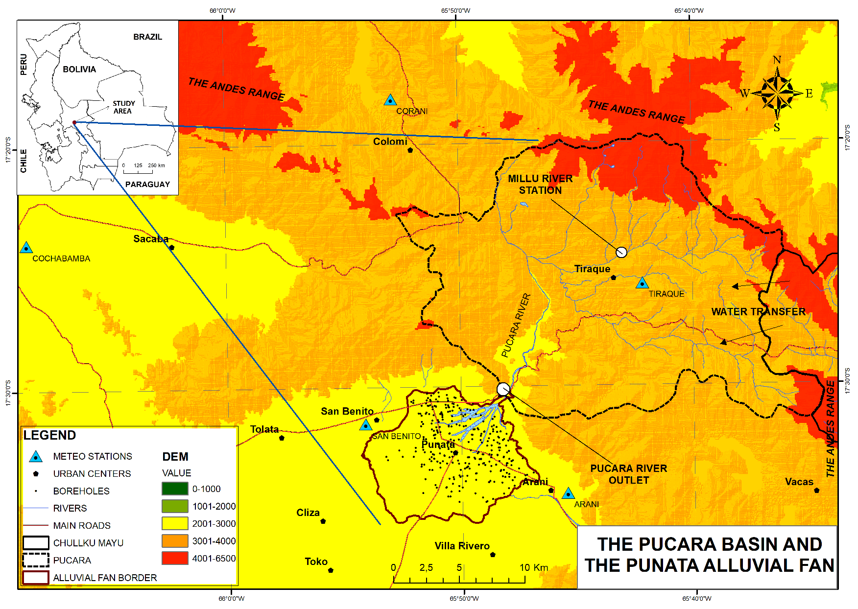
In Bolivia, warming conditions have already caused severe problems in the recent years. During 2015 and 2016, the second largest lake in Bolivia, Poopo lake, dried up completely [22,23]. During these years, the main cities of Bolivia suffered from water supply shortages affecting more than 3 million inhabitants. In rural and sub-urban areas, conflicts between farmers and private water supply companies have increased [24]. One of the most important basins in central Bolivia in terms of ecological and socioeconomic aspects is the Pucara watershed system [25], which is located in the central Andes (Figure 1). This watershed consists of: (i) the Pucara basin; (ii) the Chullku Mayu basin, which is the east neighboring basin of Pucara, and from where water is transferred through artificial channels to lakes and rivers in the northeastern part of the Pucara basin; and (iii) the Punata alluvial fan, where water from the Pucara River is discharged and used for irrigation. Therefore, this study area is an integrated system including different basins [26]. It is an interesting region for research purposes, as it crosses several ecosystems (i.e., Andean, tropical Andean and sub-Andean valleys). The upper part of the system has common limits with the Amazon watershed and is considered as a wet zone due to high rates of precipitation (i.e., >2000 mm year−1). In contrast, the lower part of the system, which ends at the outer boundaries of the Punata alluvial fan, is semiarid, with low precipitation rates (i.e., <500 mm year−1). The Punata fan is a region with a growing urban area, coexisting with intensive agricultural production. The increasing demand of water access generates a great urgency to study the effects of climate variability in this system in order to strengthen mechanisms of management, regulation, and planning of water use.
Previous hydrogeological studies in the area have not analyzed possible impacts of climate variability on the water resources of the region. The aim of this paper is therefore to identify the climate variability in terms of annual precipitation and whether this variability has any significance to the groundwater regime. Such understanding would assist in formulating better groundwater management policies.
2. Methods
2.1. Study Area
The study area is situated in the central part of Bolivia within the Andes region, specifically in the sub-Andean Valleys of the department of Cochabamba, Bolivia (Figure 1), between the coordinates 17°38′–17°25′ S and longitude 65°55′–65°35′ W. The Pucara basin has an approximate area of 440 km2. Important lakes are located at the highest parts of the basin, and the water from these lakes is drained through artificial channels and rivers to the irrigation areas in the Punata alluvial fan. Some of these lakes are filled through artificial channels with water coming from the neighboring Chullku Mayu basin. The elevation of the Pucara basin ranges from 4650 m above sea level (m a.s.l.) in the eastern part of the Andes range, to about 2800 m a.s.l. in the southern part of the basin.
The Punata alluvial fan is located downstream the outlet of the Pucara basin and extends over an area of 90 km2. The alluvial fan is flanked to the north and east by the Pucara basin. From the southeast to the west, a clay fringe limits the fan and potentially represents the lateral boundary of the aquifer system. The topography is mainly northeast-southwest gently sloping with an altitude of approximately 2700 m a.s.l. The climate in the Punata fan is semiarid with an average precipitation of 350 mm year−1. The main source for water supply comes from groundwater, which is expected to be mainly recharged by the Pucara River [27]. This river represents the main stream of the study area. It starts from the heights of the Pucara basin (4650 m a.s.l.) and flows downstream until it discharges in the Punata alluvial fan.
The regional and local geology is described in the project by the United Nations Development Program (UNDP) and the Geology Service of Bolivia (GEOBOL) [28]. The mountainous region is formed by Ordovician rocks, while the valleys are filled with unconsolidated Quaternary sediments. The main Quaternary units are described in Gonzales Amaya et al. [29] and are: alluvial fan, fluvial, fluvio-lacustrine, and terrace deposits. These deposits range from coarse material close to the mountain massif and outlet of rivers, to fine sediments in the center of the basin.
The groundwater system in the Punata fan is generally unconfined close to the apex of the fan, and it is semiconfined to confined towards the middle and distal part of the fan [28]. The depth of the water table ranges between 10 and 15 m in the distal part of the fan, to 35 and 40 m in the head of the fan. Yields from boreholes range from less than 0.5 L/s in the distal part of the fan to 18 L/s in the upper part of the fan. The high porosity in the alluvial fan and fluvial deposits make them good areas for water infiltration, and in these deposits is where the Pucara River discharges its water. Hence, the existence of a direct relationship between the river and aquifer it is expected.
2.2. Data Collection
There are several meteorological stations within and close to the study area. However, only four have long time series (i.e., >30 years). These stations, which are marked by triangles in Figure 1, are San Benito (2710 m a.s.l.), Cochabamba (2560 m a.s.l.), Tiraque (3280 m a.s.l.), and Corani (3320 m a.s.l.). The San Benito and Cochabamba stations are located in valley regions where the climate is mostly semiarid, while the Tiraque and Corani stations are located in mountainous regions where the climate is much wetter. The precipitation data used for this study were recorded on a daily basis. The quality of the data was evaluated with quantitative methods such as the double mass curve. Missing data were completed by applying multiple regression with regional stations and daily data. The time records are displayed in Table 1, and the coordinates and elevation of each meteorological station are also listed.
Apart from meteorological information, data have been collected from a hydrological study of the Pucara basin [30], that used a deterministic hydrological model for the estimation of river flows, i.e., precipitation, evapotranspiration, runoff, and soil cover were the main input variables. The results include simulated Pucara River discharges from 1965 to 2008, which provide insights on how river flow variations can affect the aquifer recharge in the Punata alluvial fan. The quality control of the meteorological series was done through an analysis of consistence and homogenization. The data gaps were again filled by multiple regression. Two hydrometric stations were used for calibration and validation of the river flow: the Millu River station in the highlands of the Pucara basin, and the Pucara River station located in the outlet of the basin (Figure 1). After considering 9 years of daily data, the calibration and validation of the river flow model yielded R2 values of 0.8 and 0.7, respectively. Finally, historical levels of groundwater table were gathered. During 2011 and 2012, a total of 27 boreholes were monitored by the University Mayor de San Simon in Cochabamba, Bolivia. This was done at a weekly time step. Moreover, automatic groundwater level monitoring devices were installed in four wells. The time resolution of these automatic monitoring devices was hourly from November 2015 to August 2016. The locations of the selected groundwater monitoring well are listed in Table 1 (stations with the prefix PM).
2.3. El Niño Southern Oscillation and Southern Oscillation Index
ENSO exerts global dominant control of the interannual climate variability, where there is a strong coupling between the tropical ocean and atmosphere [15]. The Southern Oscillation Index (SOI) is a measure of ENSO, where the temporal variations in the recorded air pressure difference at sea level in the Southern Ocean Pacific between stations located in Tahiti and Darwin are expressed as a standardized index. The SOI has been considered as the starting point to study climatic anomalies in many regions of the world [31,32,33,34], particularly in the Southern Hemisphere [35,36,37,38]. For instance, during 1982–1983, atmospheric pressures above the average were recorded in Darwin, and low atmospheric pressures were recorded in Tahiti. Hence, one of the most severe El Niño events was recorded in that period, and the SOI yielded negative values [39]. In general, prolonged periods of negative SOI values coincide with atypical warmer temperatures in the Pacific Ocean (i.e., El Niño episode), while prolonged periods of positive SOI values coincide with atypical colder temperatures (i.e., La Niña episode) [40]. For this study, SOI data were accessed from the website of the Australian Government Bureau of Meteorology [41]. These data were used for delimiting strong events of El Niño and La Niña. This was done by estimating an average SOI value for each hydrological year (i.e., from September to August) of the study area, followed by applying thresholds of +8 and −8 in the SOI scale to identify strong events of El Niño and La Niña, respectively [42]. ENSO effects on the climate in South America were analyzed in other studies [43,44], where a decadal to multi-decadal variability in the frequency and type of ENSO events was observed [43,45]. For example, Meinke, et al. [46] recognized that ENSO variability is well defined within the standard period of 2.5 to 8 years; however, decadal (9 to 13 years) and interdecadal (15 to 18 years) periods are also significant for explaining ENSO variability.
2.4. Climate Variability and Trends
It is important to study the climate variability in time and space and take this into consideration for planning and forecasting possible natural hazards such as droughts and floods. In order to understand the climate variability and trends, it is necessary to study the historical records and their variations (climate oscillations). Several methods and studies exist that analyzed climate trends and natural climate variations [47,48,49,50,51,52]. Most of these studies used non-parametric methods such as Mann-Kendall and Spearman. Tabari et al. [53] explain that these methods take into consideration the rank of the measurements rather than their actual values. However, the results of these methods are often influenced by internal correlations in the time series, which increases the possibility of false trend or no-trend rejections. Consequently, the quantile perturbation method (QPM) has been used in this research. This is a method that does not depend on the above-mentioned constraints. The methodology and theory of this method are well described in [54,55,56], and this method is based on the frequency perturbation method [57,58,59].
The QPM is used in this study to analyze temporal anomalies (oscillations) in the meteorological conditions. It requires two time series: one of the series is taken as the reference or baseline series, while the other is selected as a subseries of the past. The baseline series is a long (i.e., entire) observed time series with a length of years. In this study, equals the length of the full available time series: 61, 50, 74, 63 and 136 years for Tiraque, San Benito, Cochabamba, Corani and SOI, respectively. The subseries are selected sub-periods from these total time series and represent the periods of interest with a length of years. Decadal and interdecal periods can significantly represent the oscillation periods [46]. Hence, the selection of the time window length should not be done arbitrary [60] but by taking into consideration similar observed times in the region. This study used a length of 12 years, which allowed the identification of high and low inter-annual anomalies. Other authors, e.g., Torrence and Webster [61], Mora and Willems [62], and Villazon [42], found similar times for the SOI decadal oscillation period.
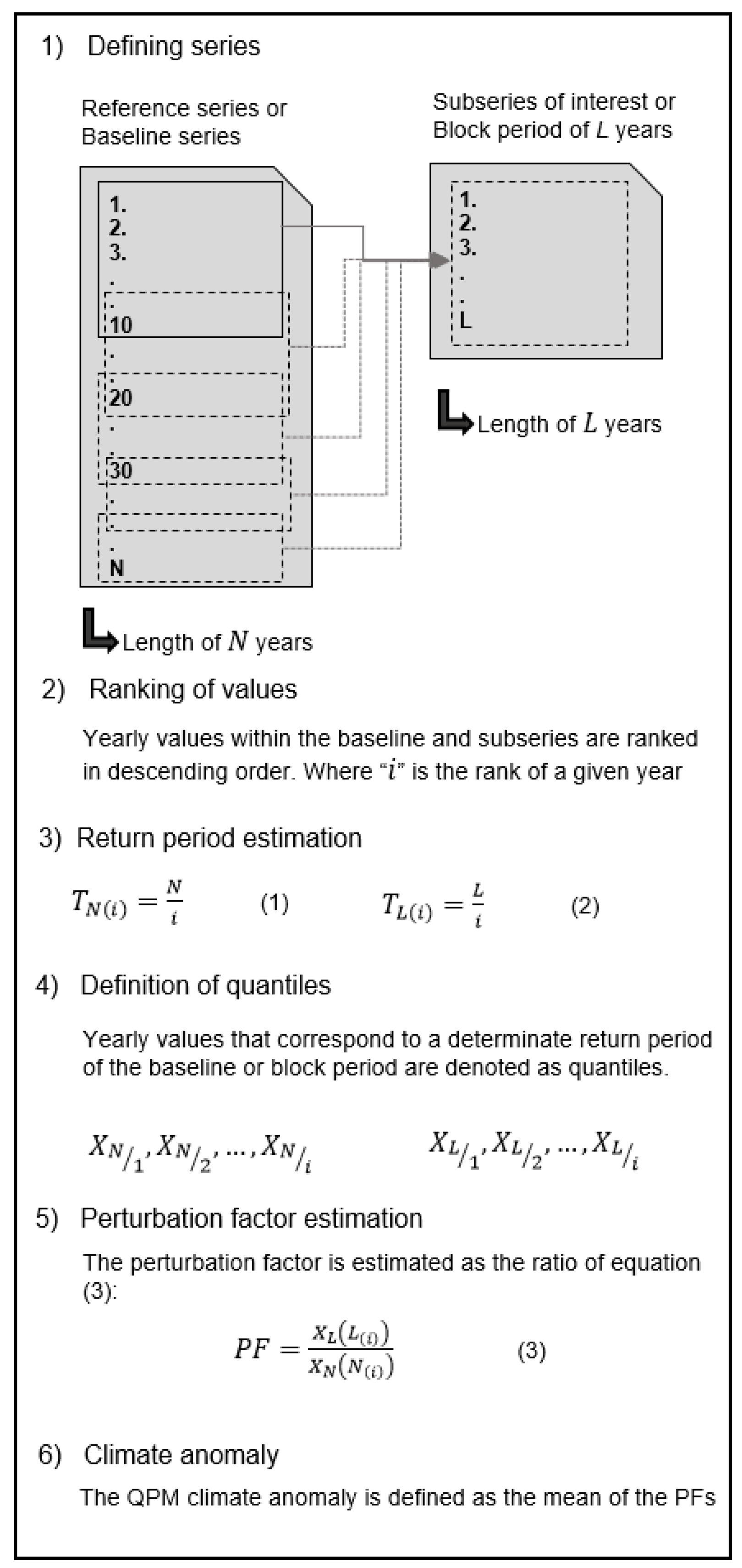
For each of the subseries, the climate anomaly is defined, which can be understood as the relative change of time series statistics derived from the subseries versus the same statistics but derived from the reference series. In the QPM, quantiles defined as the value for a given exceedance probability are considered and for all empirical exceedance probabilities above a given threshold. Depending on the selected threshold, more or less extreme conditions can be considered. The QPM climate anomaly is then defined as the mean ratio of the quantile derived from the subseries over the corresponding quantile (for the same exceedance probability) from the reference series, and for all quantiles or exceedance probabilities above the given threshold. Figure 2 shows the different steps in the estimation of the climate anomaly [53,54,62]: (1) Generate subseries with a length of years from the reference series. (2) Extract independent values from each subseries and from the reference series; in this study, annual mean values are considered; these values are ranked from the highest to the lowest value, where is the rank order. (3) Compute empirical return periods for each ranked value as the ratio of the subseries length over the rank of the extreme value. (4) The values that correspond to each return period represent the quantiles. Steps 1 to 3 are repeated for each possible subseries. (5) For each quantile, the ratio (also denoted as the ‘perturbation factor’ PF) is computed as the respective value in the subseries relative to that in the reference series with the same return period. (6) Finally, from the PF of all the considered values (years in this study), an average value is calculated for all the quantiles. This average PF is the climate anomaly. In this study, the anomalies were estimated for subseries with a length of 12 years moved with a time step of one year. Because the empirical return periods of the reference and subseries do not necessary coincide, the quantiles of the reference series () are estimated by linear interpolation of the values with closest empirical return periods [62].
The significance of the climate anomaly was determined by using a non-parametric bootstrapping method to obtain Monte Carlo confidence intervals [53,63]. Under the null hypothesis of a stationary climate, the extremes (yearly maxima in this study) are randomly reshuffled in time such that random samples are generated for each of the subseries. From these random samples, the climate anomalies are recomputed. By repeating this process numerous times (1000 times in this study), confidence intervals on the climate anomalies are computed, i.e., the 25th and 975th ranked anomaly values define the 95% confidence interval for subseries. They provide the basis for testing for each subseries the null hypothesis of no significant changes in climate statistics (extreme quantiles in this case) [53,63,64].
In this study, the QPM method is applied first in the SOI in order to assess and determine the applicability of this method for identifying oscillation patterns. Then, if patterns are detected in the SOI series, and under the assumption that there is a teleconnection between SOI and precipitation in the Pucara region, the QPM is applied in the study area for the detection of oscillation patterns in precipitation.
3. Results and Discussion
3.1. Climate Variability
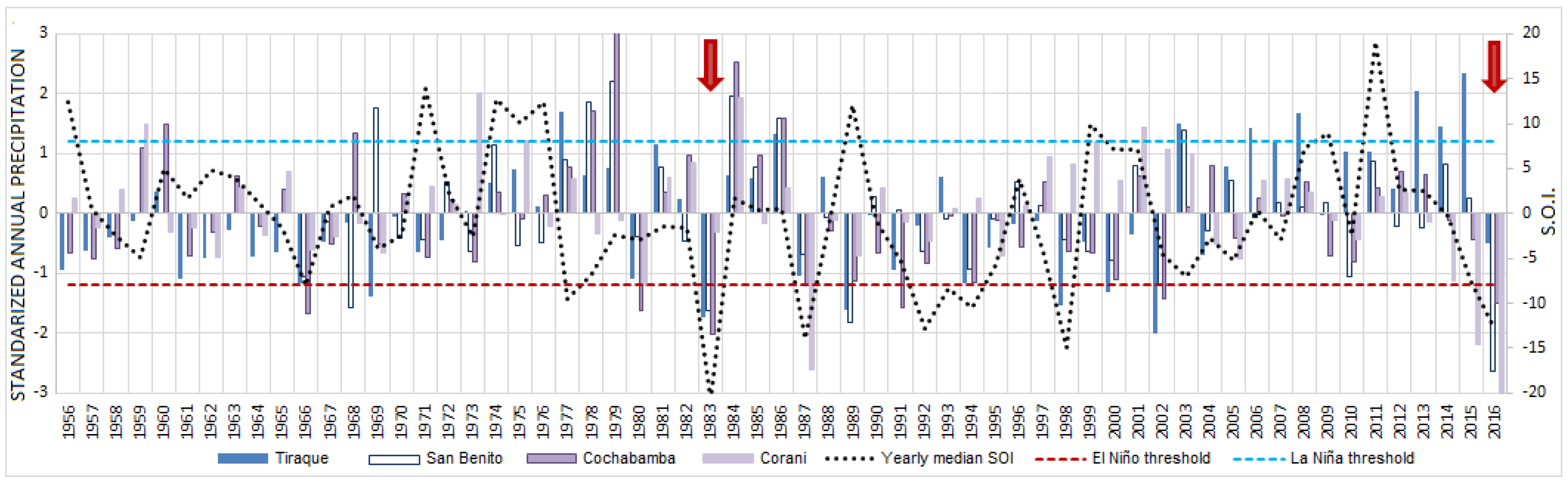
In Figure 3, the annual normalized precipitation of the different meteorological stations is plotted. The yearly average of the SOI values, and the limits of high El Niño and La Niña events are displayed as well. Two strong events of El Niño are indicated by arrows. The event around the year 1983 was ranked by many authors as the strongest El Niño ever recorded in the last decades [39,65,66]. In years around an El Niño event, all the meteorological stations recorded low precipitation, which is in agreement with the El Niño characteristics of the region. During the recent years, 2015 to 2016, unusually dry periods were observed in many parts of Bolivia, leading to severe droughts [22,23], and this is explained by the negative phase of the SOI (i.e., a strong El Niño event is taking place).
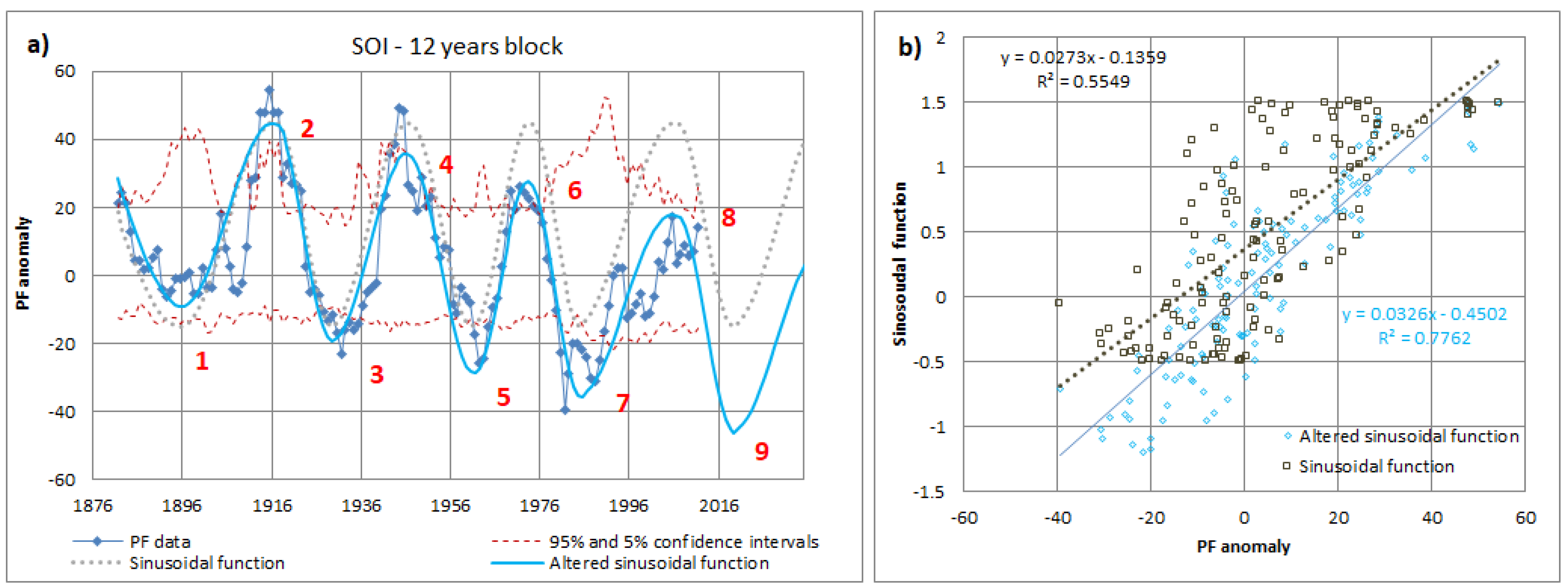
Figure 4a shows that after computing the QPM climate anomaly using the SOI series, an oscillatory behavior is obtained. After applying a dynamic sinusoidal function, it is shown to be quasi cyclic. The sinusoidal period, however, varies in time: from 28 years to 33 years. After adjusting the function based on the long-term decreasing trend, the altered sinusoidal function yields an R2 close to 0.78 (Figure 4b). The SOI oscillations show 4 marked cycles of El Niño events, and 4 cycles of La Niña events (odd and even numbers in Figure 4a, respectively) that took place in the past. Again, it is possible to distinguish the El Niño events from 1983 and 2015. The QPM hence clearly filters out and visualizes these patterns. Based on the 95% confidence intervals, the most extreme oscillation high and low periods are found to be significant. Several of the highest and lowest anomalies during oscillations high and low periods indeed cross the confidence interval bounds.
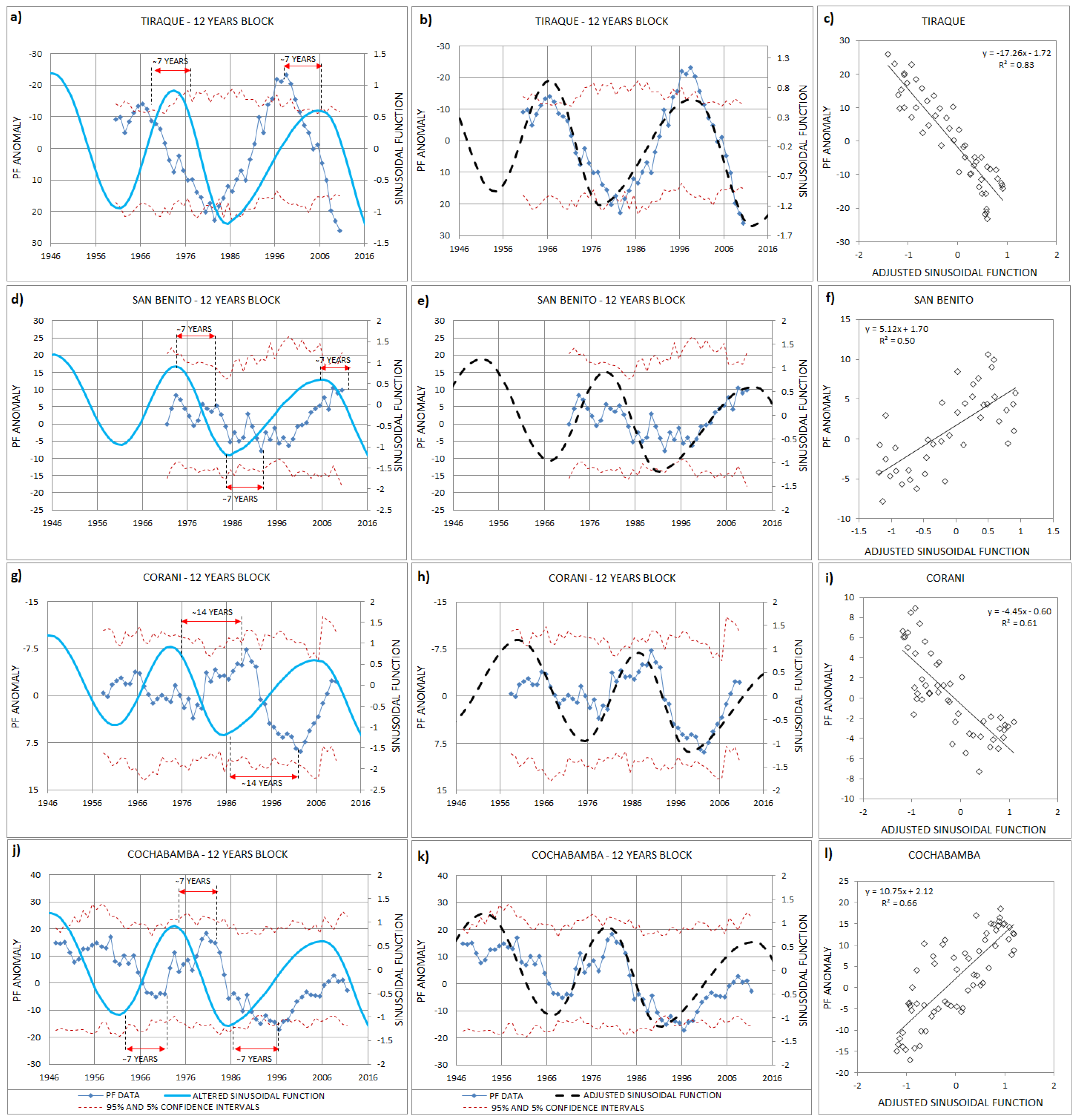
The QPM methodology was applied to the annual precipitation at Tiraque, San Benito, Corani and Cochabamba stations (Figure 5). The teleconnection between ENSO and precipitation in the study area was assessed using the QPM. In general, there is a similar oscillatory behavior of the precipitation and ENSO based climate anomalies, but with a phase shift. This indicates a delayed response of the precipitation anomaly to the SOI anomaly. Parker, et al. [45] noted that ENSO might have lagged signatures in some tropical processes in the off-equatorial ocean, hence it might affect the frequency of El Niño and La Niña events. Therefore, a phase shift in the study area might happen due to some delayed processes elsewhere. The mean phase shift required to obtain a close match of the altered SOI-based sinusoidal function with the precipitation-based anomalies equals approximately 7 years (Figure 5d,j) for the stations that are located in the inter-Andean valley with an altitude less than 3000 m a.s.l. (e.g., San Benito and Cochabamba). For the other two stations that are located at altitudes higher than 3000 m a.s.l. and close to the tropical region, the relationship shows a negative correlation, and the PF Anomaly values are in reverse order.
For Tiraque station, there is a negative shift of 7 years and for the Corani station, the shift is positive but is 14 years. It is not possible to think that all the shifts are going to be equal and the correlation will be in the same direction because of randomness and uncertainty (i.e., precipitation is a stochastic process). There is also a similarity in the oscillatory behavior of the precipitation anomalies at the different stations, which respond similarly to the ENSO influence. In this respect, Tiraque and Corani stations show similar patterns for the precipitation anomalies, and Cochabamba and San Benito stations also showed analogous patterns between each other. Cochabamba and San Benito are stations in a subregion with semiarid conditions that show the strongest influence on the positive phase of the SOI (the La Niña events). Corani and Tiraque are stations in another subregion with wetter conditions that show the strongest influence on the negative phase of the SOI (the El Niño events).
According to these results it can be suggested that ENSO effects are temporally and spatially correlated with the precipitation in the Pucara basin and the Punata alluvial fan. It is clear that these climate anomalies might affect socioeconomic activities based on water usage such as agriculture or industry, and increase the risk of water shortages. Similar results were obtained by Miranda [39] for the central part of Bolivia. The knowledge about the phase shifts between the precipitation and the SOI anomalies can be used for further planning. By studying the trend of the SOI-based anomaly, the delayed changes in mean annual precipitation conditions can be anticipated. However, for doing so, it is necessary to assure that the applied series are homogeneous and consistent [67].
The statistical significance of the anomalies in the Tiraque station for the high and low oscillation of the precipitation appear significant at the 5% significance level. However, given the similarity in timing at the different stations and the correlation with the SOI, it is expected that this is due to the relatively short data records (relatively short in comparison with the length of the oscillation periods).
3.2. Groundwater Response to Rainfall Variability
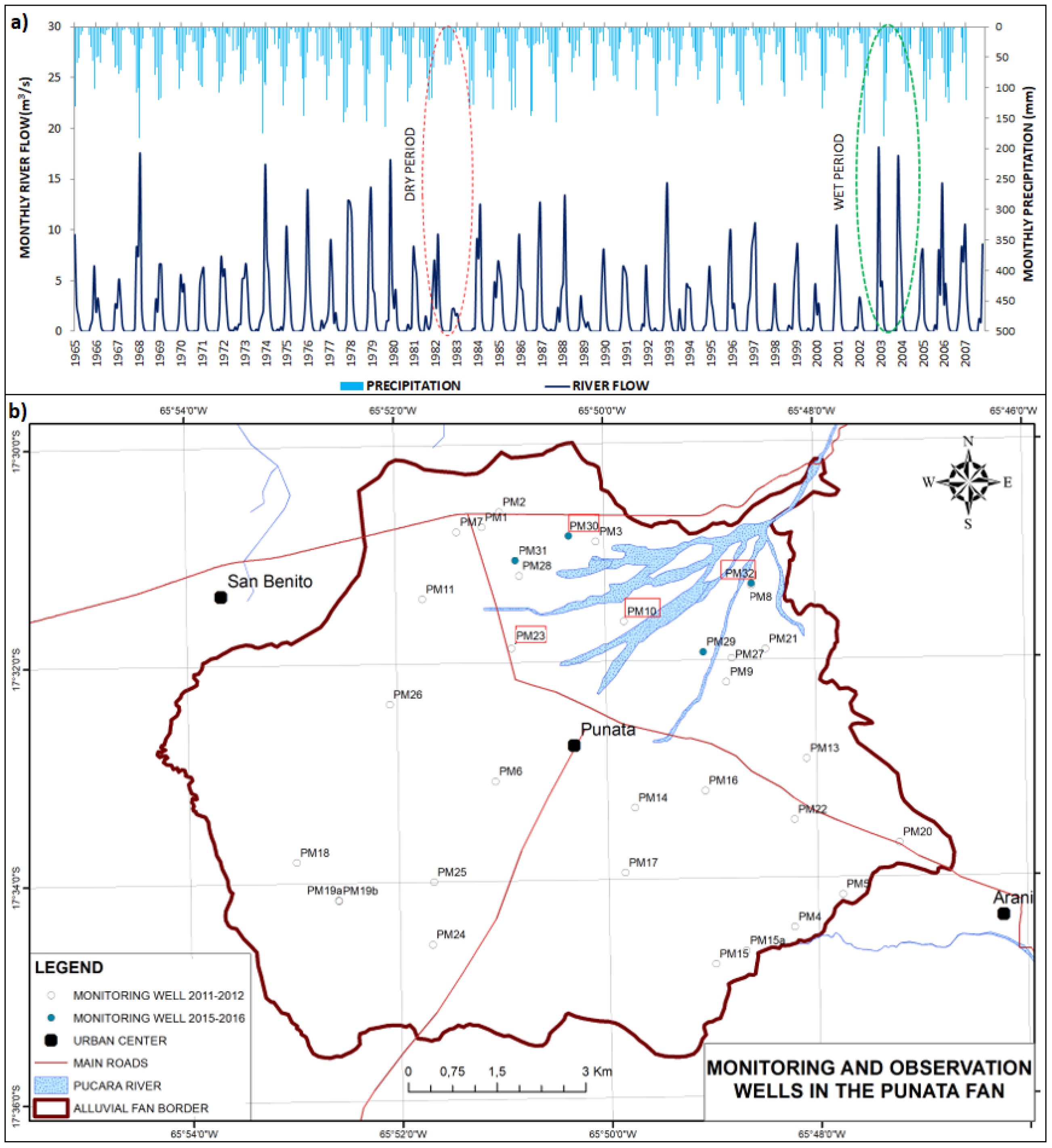
The Punata alluvial fan is an area with an extensive agriculture and with local groundwater as the main water supply. Gonzales Amaya and Barmen [27] indicated that one of the main recharge sources of the local aquifer is the Pucara River. In order to transfer the temporal precipitation variations to corresponding groundwater table variations, hydrological and hydraulic modeling is used. Figure 6a shows the Pucara River flow at the outlet of the basin and the precipitation at the Tiraque station. This meteorological station is located in the central part of the Pucara basin, and it may be assumed that the precipitation in other parts of the basin is similar to that at the Tiraque station.
From Figure 6a, it can be suggested that precipitation is the main source for recharging the river flow, as increasing/decreasing trends in precipitation yield increasing/decreasing trends in river flow. Chen et al. [68] stated that climate change can alter the pattern of runoff, the frequency and severity of floods, and emphasize that if in arid or semi-arid regions (e.g., the Punata alluvial fan) small changes in precipitation and temperature occur, these might result in marked changes in runoff. This effect is well illustrated when monthly average precipitation at Tiraque station from years 1983 and 2003 is compared with the monthly average Pucara River flow in the same periods. During 1983 (i.e., dry period), the monthly average precipitation was 25.1 mm and the monthly average river flow was 0.7 m3. While during 2003 (i.e., wet period), the monthly average precipitation was 43.2 mm and the monthly average river flow was 2.8 m3. Both periods are illustrated and encircled in Figure 6a.
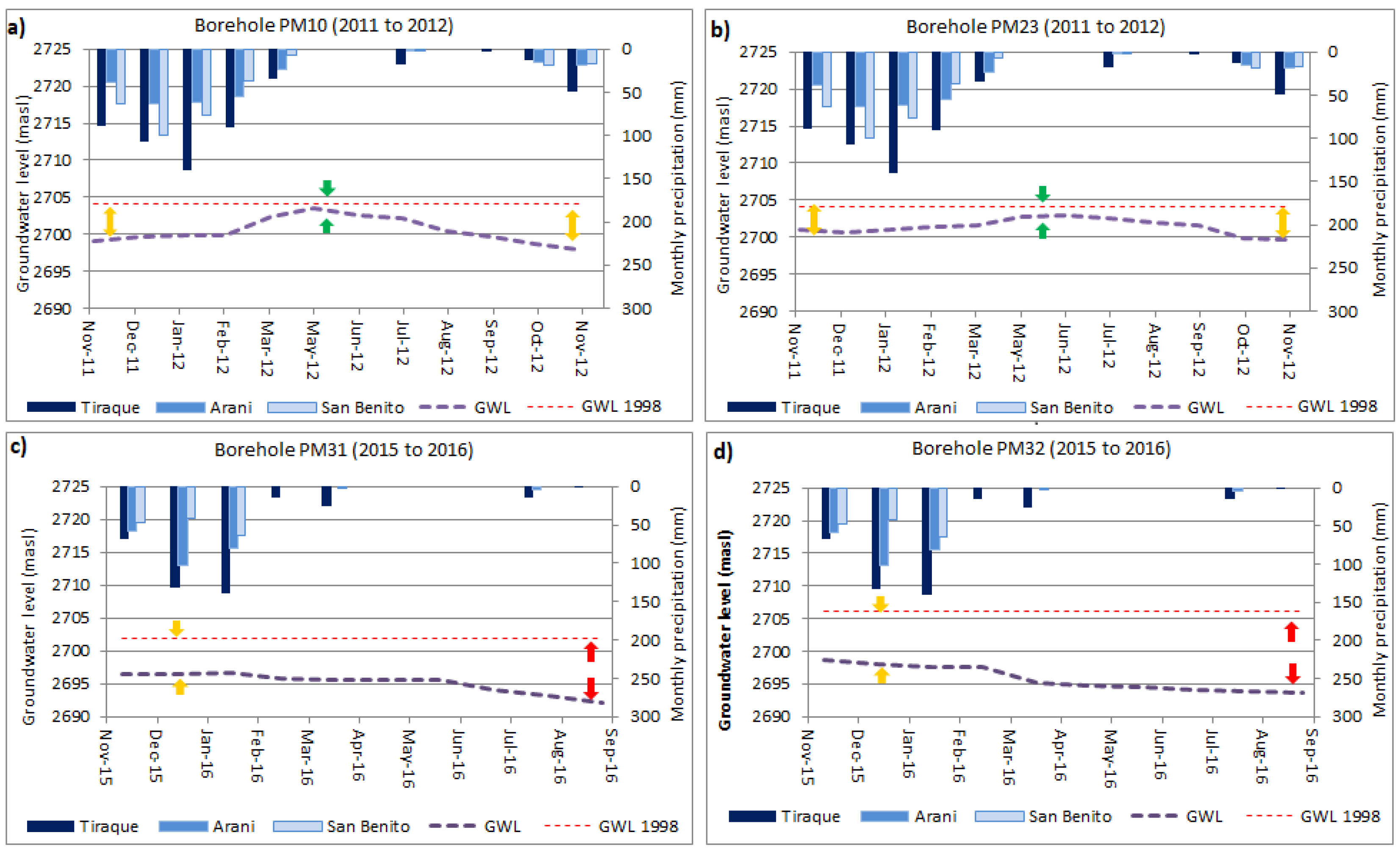
Further analysis was conducted using the groundwater table records available for the period 2011–2012 at 29 groundwater wells and the additional recordings for 2015–2016 based on installed automatic groundwater table recording stations in four boreholes (see their locations in Figure 6b). Figure 7 displays the groundwater table fluctuation in the Punata aquifer for four selected monitoring stations. Because these stations are close to the Pucara River outlet, and close to each other, the groundwater levels are expected to be similar. Moreover, the location of the four selected monitoring stations is placed close to the Pucara River and within alluvial fan and fluvial deposits. These deposits are formed of coarser materials, which means that it is expected that river flow infiltrates relatively rapid and recharges the aquifer system. In order to asses if any substantial change has occurred, compared with historic recorded levels, the annual average groundwater table of 1998 [69] is plotted in all the four selected stations (Figure 7).
During the yearly rainy season, i.e., October to March (Figure 7), groundwater is not extracted and, therefore, it is expected that the groundwater table rises. It is during this season that heavy precipitation can occur, leading to flash floods in the Pucara River. These heavy floods can rapidly increase the groundwater recharge rate in the Punata fan. On the contrary, during the yearly dry season (April to September) groundwater is pumped out and it is expected that groundwater levels start to decrease.
Figure 7 shows based on monitoring stations PM10 and PM23 that during the rainy season the groundwater table rises, and that it decreases during the dry season. It is also shown that the maximum groundwater table peak during 2011–2012 is slightly below the annual average for 1998. The groundwater levels at monitoring stations PM31 and PM32 differ from such patterns. During and after the rainy season, there are no clear trends of increasing groundwater levels. It is moreover shown that the difference in groundwater levels between 2015–2016 and 1998 is higher than in 2011–2012. These variations in groundwater levels might be explained by the climate variability of the area. During the period 2015–2016, the SOI values tend to be negative, which is an indicator that an El Niño event is taking place; therefore, a dry period is expected with low rates of precipitation and thus the Pucara River flow and the groundwater recharge in the Punata fan will decrease. On the other hand, a positive SOI anomalous period might result in wet years, which means that the Pucara River does recharge the aquifer with higher rates leading to an increase in groundwater levels. Another reason which might assist in understanding the decrease of the groundwater table is that since recent years, the number of wells has increased considerably in the study area. Therefore, more groundwater was pumped out during the period 2015–2016 than during 2011–2012 and 1998. Both climate variability and overexploitation must be analyzed and discussed with the local actors, in order to implement mitigation plans and sustainable management strategies.
4. Conclusions
In this study, the climate variability in the Pucara basin and the Punata alluvial fan was investigated using the QPM approach for analyzing (multi-)decadal anomalies in precipitation conditions and their correlation with large-scale drivers such as the SOI. Results suggest that there is a strong temporal variability, with semi-cyclic oscillation patterns of periods of 28 to 33 years in rainfall events, based on a 12-year sliding window. The research showed that extreme SOI conditions influence the precipitation regime of the study area. After a very low phase of the SOI oscillation, dry conditions appear to occur in the Pucara basin, leading to reduced recharge and groundwater table levels for the Punata fan. However, positive phases of the SOI oscillation lead to wet conditions in the Pucara basin and increase the recharge and groundwater levels in the Punata fan. This relationship between changes in the phase of the SOI and precipitation in the study areas indicates that there is teleconnection between them. The association of El Niño events with low precipitation is in agreement with Miranda [39] and Villazon [42].
The groundwater level observations in the Punata alluvial fan suggest that they might be influenced by the inflow of Pucara River. When the groundwater levels of 2011–2012 and 2015–2016 are compared with the average level of 1998, it appears that the level differences are increasing with time. This might be explained by climate variability, due to the more wet period around 1998 which increased the groundwater levels, and the drier conditions during 2011–2012 and 2015–2016 with lower groundwater recharge rates. Another factor that may have played a significant role and that deserves further investigation is the more intense groundwater overexploitation in the recent years.
Estimates of the actual recharge-discharge rates are recommended to determine if the groundwater exploitation has equaled or exceeded the groundwater recharge rate. Also, longer time series of groundwater level observation are needed in order to confirm the link between rainfall variability and groundwater level fluctuations. Therefore, a groundwater level dataset that extends beyond one calendar year would greatly improve the correlation between presented climate signals and any potential groundwater response. This information might assist in determining the real effects of climate variability on the Punata fan groundwater. Appropriate land use, adequate policies of groundwater system protection, continuous monitoring of groundwater levels, and awareness of climate variability are keys to guarantee sustainability of groundwater and are particularly important during periods of extreme climatic conditions (i.e., dry periods) when there is a reduced access to water.
Author Contributions
A.G.A. conceived the research and collected the data; A.G.A., M.F.V. and P.W. analyzed and wrote the paper.
Acknowledgments
The present study was supported by the Swedish International Development Agency (SIDA) in collaboration with Lund University (Sweden), and Universidad Mayor de San Simon (Bolivia). We are grateful for all the support received. Special thanks are extended to Centro Agua for providing information regarding groundwater levels and to all students who collaborated during the field work.
Conflicts of Interest
The authors declare no conflict of interest.
References
- Russo, T.A.; Lall, U. Depletion and response of deep groundwater to climate-induced pumping variability. Nat. Geosci. 2017, 10, 105–108. [Google Scholar] [CrossRef]
- Molina-Navarro, E.; Hallack-Alegría, M.; Martínez-Pérez, S.; Ramírez-Hernández, J.; Mungaray-Moctezuma, A.; Sastre-Merlín, A. Hydrological modeling and climate change impacts in an agricultural semiarid region. Case study: Guadalupe river basin, Mexico. Agric. Water Manag. 2016, 175, 29–42. [Google Scholar] [CrossRef]
- Abu-Allaban, M.; El-Naqa, A.; Jaber, M.; Hammouri, N. Water scarcity impact of climate change in semi-arid regions: A case study in Mujib Basin, Jordan. Arab. J. Geosci. 2015, 8, 951–959. [Google Scholar] [CrossRef]
- Marengo, J.A.; Jones, R.; Alves, L.M.; Valverde, M.C. Future change of temperature and precipitation extremes in South America as derived from the precis regional climate modeling system. Int. J. Climatol. 2009, 29, 2241–2255. [Google Scholar] [CrossRef]
- Haylock, M.R.; Peterson, T.; Alves, L.; Ambrizzi, T.; Anunciação, Y.; Baez, J.; Barros, V.; Berlato, M.; Bidegain, M.; Coronel, G. Trends in total and extreme South American rainfall in 1960–2000 and links with sea surface temperature. J. Clim. 2006, 19, 1490–1512. [Google Scholar] [CrossRef]
- Nobre, P.; Shukla, J. Variations of sea surface temperature, wind stress, and rainfall over the tropical Atlantic and South America. J. Clim. 1996, 9, 2464–2479. [Google Scholar] [CrossRef]
- Grimm, A.M.; Tedeschi, R.G. Enso and extreme rainfall events in South America. J. Clim. 2009, 22, 1589–1609. [Google Scholar] [CrossRef]
- Andrade, M.F. La Economía del Cambio Climático en Bolivia: Validación de Modelos Climáticos; Inter-American Development Bank: Washington, DC, USA, 2014. [Google Scholar]
- Wolter, K.; Timlin, M.S. El niño/southern oscillation behaviour since 1871 as diagnosed in an extended multivariate enso index (mei. Ext). Int. J. Climatol. 2011, 31, 1074–1087. [Google Scholar] [CrossRef]
- Trenberth, K.E.; Hoar, T.J. The 1990–1995 el niño-southern oscillation event: Longest on record. Geophys. Res. Lett. 1996, 23, 57–60. [Google Scholar] [CrossRef]
- Coelho, C.; Uvo, C.; Ambrizzi, T. Exploring the impacts of the tropical pacific sst on the precipitation patterns over South America during enso periods. Theor. Appl. Climatol. 2002, 71, 185–197. [Google Scholar] [CrossRef]
- Barros, V.R.; Doyle, M.E.; Camilloni, I.A. Precipitation trends in southeastern South America: Relationship with enso phases and with low-level circulation. Theor. Appl. Climatol. 2008, 93, 19–33. [Google Scholar] [CrossRef]
- Caviedes, C.; Waylen, P.R. Respuestas del clima de américa del sur a las fases de enso. Bull. L'Inst. Fr. D'études Andines 1998, 27, 613–626. [Google Scholar]
- Grimm, A.M. Interannual climate variability in South America: Impacts on seasonal precipitation, extreme events, and possible effects of climate change. Stoch. Environ. Res. Risk Assess. 2011, 25, 537–554. [Google Scholar] [CrossRef]
- Aceituno, P. On the functioning of the southern oscillation in the South American sector. Part I: Surface climate. Mon. Weather Rev. 1988, 116, 505–524. [Google Scholar] [CrossRef]
- Ramírez, E.; Francou, B.; Ribstein, P.; Descloitres, M.; Guérin, R.; Mendoza, J.; Gallaire, R.; Pouyaud, B.; Jordan, E. Small glaciers disappearing in the tropical andes: A case-study in bolivia: Glaciar chacaltaya. J. Glaciol. 2001, 47, 187–194. [Google Scholar] [CrossRef]
- Bradley, R.S.; Vuille, M.; Diaz, H.F.; Vergara, W. Threats to water supplies in the tropical andes. Science 2006, 312, 1755–1756. [Google Scholar] [CrossRef] [PubMed]
- Escurra, J.J.; Vazquez, V.; Cestti, R.; De Nys, E.; Srinivasan, R. Climate change impact on countrywide water balance in bolivia. Reg. Environ. Chang. 2014, 14, 727–742. [Google Scholar] [CrossRef]
- Vuille, M.; Francou, B.; Wagnon, P.; Juen, I.; Kaser, G.; Mark, B.G.; Bradley, R.S. Climate change and tropical Andean Glaciers: Past, present and future. Earth-Sci. Rev. 2008, 89, 79–96. [Google Scholar] [CrossRef]
- Urrutia, R.; Vuille, M. Climate change projections for the tropical andes using a regional climate model: Temperature and precipitation simulations for the end of the 21st century. J. Geophys. Res. Atmos. 2009, 114. [Google Scholar] [CrossRef]
- Vuille, M.; Bradley, R.S.; Werner, M.; Keimig, F. 20th century climate change in the tropical andes: Observations and model results. In Climate Variability and Change in High Elevation Regions: Past, Present & Future; Springer: Berlin, Germany, 2003; pp. 75–99. [Google Scholar]
- Satgé, F.; Espinoza, R.; Zolá, R.P.; Roig, H.; Timouk, F.; Molina, J.; Garnier, J.; Calmant, S.; Seyler, F.; Bonnet, M.-P. Role of climate variability and human activity on poopó lake droughts between 1990 and 2015 assessed using remote sensing data. Remote Sens. 2017, 9, 218. [Google Scholar] [CrossRef]
- Allen, J. Bolivia’s Lake Poopó Disappears. Available online: https://earthobservatory.nasa.gov/NaturalHazards/view.php?id=87363 (accessed on 16 March 2017).
- Wutich, A.; Ragsdale, K. Water insecurity and emotional distress: Coping with supply, access, and seasonal variability of water in a Bolivian squatter settlement. Soc. Sci. Med. 2008, 67, 2116–2125. [Google Scholar] [CrossRef] [PubMed]
- Saldías, C.; Boelens, R.; Wegerich, K.; Speelman, S. Losing the watershed focus: A look at complex community-managed irrigation systems in Bolivia. Water Int. 2012, 37, 744–759. [Google Scholar] [CrossRef]
- Saldías, C.; Speelman, S.; Van Huylenbroeck, G. Access to irrigation water and distribution of water rights in the abanico punata, Bolivia. Soc. Nat. Resour. 2013, 26, 1008–1021. [Google Scholar] [CrossRef]
- Gonzales Amaya, A.; Barmen, G. Recharge process and origin of saline water in the semi-arid punata alluvial fan in Bolivia. Hydrol. Process. 2018, in press. [Google Scholar]
- UNDP-GEOBOL. Proyecto Integrado de Recursos Hidricos Cochabamba (Integrated Water Resources Project Cochabamba); United Nations Development Programme: Cochabamba, Bolivia, 1978. [Google Scholar]
- Gonzales Amaya, A.; Dahlin, T.; Barmen, G.; Rosberg, J.-E. Electrical resistivity tomography and induced polarization for mapping the subsurface of alluvial fans: A case study in Punata (Bolivia). Geosciences 2016, 6, 51. [Google Scholar] [CrossRef]
- Cruz, R. Technical Report: Hidrological Study of the Tiraque Valley (Estudio Hidrologico del Valle de Tiraque-Informe Final); Universidad Mayor de San Simon: Cochabamba, Bolivia, 2008. [Google Scholar]
- Keppenne, C.L.; Ghil, M. Adaptive filtering and prediction of the southern oscillation index. J. Geophys. Res. Atmos. 1992, 97, 20449–20454. [Google Scholar] [CrossRef]
- An, S.-I.; Bong, H. Inter-decadal change in el niño-southern oscillation examined with bjerknes stability index analysis. Clim. Dyn. 2016, 47, 967–979. [Google Scholar] [CrossRef]
- Kosaka, Y.; Xie, S.-P. Recent global-warming hiatus tied to equatorial pacific surface cooling. Nature 2013, 501, 403–407. [Google Scholar] [CrossRef] [PubMed]
- Allen, J.T.; Tippett, M.K.; Sobel, A.H. Influence of the el niño/southern oscillation on tornado and hail frequency in the United States. Nat. Geosci. 2015, 8, 278–283. [Google Scholar] [CrossRef]
- Grimm, A.M.; Barros, V.R.; Doyle, M.E. Climate variability in southern South America associated with el niño and la niña events. J. Clim. 2000, 13, 35–58. [Google Scholar] [CrossRef]
- Biondi, F.; Gershunov, A.; Cayan, D.R. North pacific decadal climate variability since 1661. J. Clim. 2001, 14, 5–10. [Google Scholar] [CrossRef]
- Deser, C.; Phillips, A.S.; Hurrell, J.W. Pacific interdecadal climate variability: Linkages between the tropics and the North Pacific during boreal winter since 1900. J. Clim. 2004, 17, 3109–3124. [Google Scholar] [CrossRef]
- Murphy, B.F.; Power, S.B.; McGree, S. The varied impacts of el niño–Southern Oscillation on Pacific island climates. J. Clim. 2014, 27, 4015–4036. [Google Scholar] [CrossRef]
- Miranda, G. La influencia del fenómeno el niño y del índice de oscilación del sur en las precipitaciones de Cochabamba, Bolivia. Bull. Inst. Fr. Études Andines 1998, 27, 709–720. [Google Scholar]
- NOAA. Southern Oscillation Index (Soi). Available online: https://www.ncdc.noaa.gov/teleconnections/enso/indicators/soi/ (accessed on 22 March 2016).
- AGBM. Southern Oscillation Index (Soi) Since 1876. Available online: http://www.bom.gov.au/climate/current/soihtm1.shtml (accessed on 20 February 2016).
- Villazon, M.F. Looking for climate variability, trends and effects of El Niño event (2015–2016) in Bolivia. In XVI Congreso Bolivariano de Ingenieria Sanitaria, Medio Ambiente y Energias Renovables; ABIS: Santa Cruz, Bolivia, 2015. [Google Scholar]
- Holbrook, N.J.; Brown, J.; Davidson, J.; Feng, M.; Hobday, A.; Lough, J.; McGregor, S.; Power, S.; Riseby, J. El Niño–Southern Oscillation. In Marine Climate Change in Australia: Impacts and Adaptation Responses; CSIRO: Camberra, Austrailia, 2012. [Google Scholar]
- Quinn, W.H.; Neal, V.T.; Antunez de Mayolo, S.E. El niño occurrences over the past four and a half centuries. J. Geophys. Res. Oceans 1987, 92, 14449–14461. [Google Scholar] [CrossRef]
- Parker, D.; Folland, C.; Scaife, A.; Knight, J.; Colman, A.; Baines, P.; Dong, B. Decadal to multidecadal variability and the climate change background. J. Geophys. Res. Atmos. 2007, 112. [Google Scholar] [CrossRef]
- Meinke, H.; DeVoil, P.; Hammer, G.L.; Power, S.; Allan, R.; Stone, R.C.; Folland, C.; Potgieter, A. Rainfall variability at decadal and longer time scales: Signal or noise? J. Clim. 2005, 18, 89–96. [Google Scholar] [CrossRef]
- Casanueva, V.A.; Rodríguez Puebla, C.; Frías Domínguez, M.D.; González Reviriego, N. Variability of extreme precipitation over europe and its relationships with teleconnection patterns. Hydrol. Earth Syst. Sci. 2014, 18, 709–725. [Google Scholar] [CrossRef]
- Diaz, H.F.; Quayle, R.G. The climate of the united states since 1895: Spatial and temporal changes. Mon. Weather Rev. 1980, 108, 249–266. [Google Scholar] [CrossRef]
- Frankignoul, C.; Hasselmann, K. Stochastic climate models, part ii application to sea-surface temperature anomalies and thermocline variability. Tellus 1977, 29, 289–305. [Google Scholar] [CrossRef]
- Hamed, K.H.; Rao, A.R. A modified mann-kendall trend test for autocorrelated data. J. Hydrol. 1998, 204, 182–196. [Google Scholar] [CrossRef]
- Karl, T.R.; Knight, R.W.; Plummer, N. Trends in high-frequency climate variability in the twentieth century. Nature 1995, 377, 217–220. [Google Scholar] [CrossRef]
- Yue, S.; Pilon, P.; Cavadias, G. Power of the mann–kendall and spearman’s rho tests for detecting monotonic trends in hydrological series. J. Hydrol. 2002, 259, 254–271. [Google Scholar] [CrossRef]
- Tabari, H.; AghaKouchak, A.; Willems, P. A perturbation approach for assessing trends in precipitation extremes across Iran. J. Hydrol. 2014, 519, 1420–1427. [Google Scholar] [CrossRef]
- Ntegeka, V.; Willems, P. Trends and multidecadal oscillations in rainfall extremes, based on a more than 100-year time series of 10 min rainfall intensities at Uccle, Belgium. Water Resour. Res. 2008, 44. [Google Scholar] [CrossRef]
- Onyutha, C.; Willems, P. Spatial and temporal variability of rainfall in the Nile basin. Hydrol. Earth Syst. Sci. 2015, 19, 2227–2246. [Google Scholar] [CrossRef]
- Willems, P. Adjustment of extreme rainfall statistics accounting for multidecadal climate oscillations. J. Hydrol. 2013, 490, 126–133. [Google Scholar] [CrossRef]
- Chiew, F.H. An overview of methods for estimating climate change impact on runoff. In Proceedings of the 30th Hydrology & Water Resources Symposium: Past, Present & Future, Launceston, Australia, 4–7 December 2006; p. 643. [Google Scholar]
- Willems, P.; Vrac, M. Statistical precipitation downscaling for small-scale hydrological impact investigations of climate change. J. Hydrol. 2011, 402, 193–205. [Google Scholar] [CrossRef]
- Mpelasoka, F.S.; Chiew, F.H. Influence of rainfall scenario construction methods on runoff projections. J. Hydrometeorol. 2009, 10, 1168–1183. [Google Scholar] [CrossRef]
- Henley, B.J.; Thyer, M.A.; Kuczera, G.; Franks, S.W. Climate-informed stochastic hydrological modeling: Incorporating decadal-scale variability using paleo data. Water Resour. Res. 2011, 47. [Google Scholar] [CrossRef] [Green Version]
- Torrence, C.; Webster, P.J. Interdecadal changes in the enso–monsoon system. J. Clim. 1999, 12, 2679–2690. [Google Scholar] [CrossRef]
- Mora, D.; Willems, P. Decadal oscillations in rainfall and air temperature in the paute river basin—Southern Andes of Ecuador. Theor. Appl. Climatol. 2012, 108, 267–282. [Google Scholar] [CrossRef]
- Moges, S.A.; Taye, M.T.; Willems, P.; Gebremichael, M. Exceptional pattern of extreme rainfall variability at urban centre of Addis Ababa, Ethiopia. Urban Water J. 2014, 11, 596–604. [Google Scholar] [CrossRef]
- Taye, M.T.; Willems, P. Temporal variability of hydroclimatic extremes in the Blue Nile Basin. Water Resour. Res. 2012, 48. [Google Scholar] [CrossRef]
- Blanco, J.L.; Díaz, M. Características oceanográficas y desarrollo de el niño 1982-83 en la zona norte de chile. Investig. Pesq. (Chile) 1985, 32, 53–60. [Google Scholar]
- Glynn, P.W. El niño-southern oscillation 1982–1983: Nearshore population, community, and ecosystem responses. Annu. Rev. Ecol. Syst. 1988, 19, 309–346. [Google Scholar] [CrossRef]
- Ahzegbobor, P.A. Assessment of soil salinity using electrical resistivity imaging and induced polarization methods. Afr. J. Agric. Res. 2014, 9, 3369–3378. [Google Scholar]
- Chen, Y.; Takeuchi, K.; Xu, C.; Chen, Y.; Xu, Z. Regional climate change and its effects on river runoff in the Tarim Basin, China. Hydrol. Process. 2006, 20, 2207–2216. [Google Scholar] [CrossRef]
- Alvarado, J.R.; Camacho, A.A.; Diaz, J.Z. Estudy for the Control and Protection of Groundwater in Valle Alto (Cpas, bo 014901/01): Technical Report; SERGEOMIN-TNO: Delft, The Netherlands, 1998; p. 260. [Google Scholar]
Figure 1.
Pucara watershed system. Meteorological stations with similar climate conditions are also shown, such as San Benito, Tiraque, Cochabamba and Corani.
Figure 1.
Pucara watershed system. Meteorological stations with similar climate conditions are also shown, such as San Benito, Tiraque, Cochabamba and Corani.

Figure 2.
Flow chart for estimating the perturbation factors.

Figure 3.
Normalized annual precipitation at Tiraque, San Benito, Corani and Cochabamba stations, and yearly SOI values. SOI values beyond the +8 or −8 limits mean that a strong La Niña or El Niño took place.
Figure 3.
Normalized annual precipitation at Tiraque, San Benito, Corani and Cochabamba stations, and yearly SOI values. SOI values beyond the +8 or −8 limits mean that a strong La Niña or El Niño took place.

Figure 4.
(a) Sinusoidal approximation of the QPM climate anomaly based on SOI data; (b) Goodness-of-fit evaluation of the original and altered sinusoidal approximation.
Figure 4.
(a) Sinusoidal approximation of the QPM climate anomaly based on SOI data; (b) Goodness-of-fit evaluation of the original and altered sinusoidal approximation.

Figure 5.
(a–l) QPM climate anomaly based on precipitation data and comparison with the altered SOI sinusoidal function (left column). Sinusoidal approximation of the QPM climate anomaly based on the precipitation data (center column). Goodness-of-fit evaluation of the original and altered sinusoidal approximation (right column). The meteorological stations from top to bottom are at Tiraque, San Benito, Corani and Cochabamba, respectively.

Figure 6.
(a) Monthly precipitation at the Tiraque station and monthly average river flow at the outlet of the Pucara basin; (b) Locations of the groundwater table monitoring wells. Enclosed labels are the boreholes used in Figure 7.
Figure 6.
(a) Monthly precipitation at the Tiraque station and monthly average river flow at the outlet of the Pucara basin; (b) Locations of the groundwater table monitoring wells. Enclosed labels are the boreholes used in Figure 7.

Figure 7.
(a,b) Selected monitoring wells during the period 2011 to 2012; (c,d) Monitoring wells during the period 2015 to 2016. For location of the monitoring wells, refer to Figure 6b. Each figure shows on top the monthly precipitation variation, while the dashed lines represents the recorded groundwater level (GWL) variation during each period and during the year 1998.


Table 1.
Recording time interval of the selected meteorological stations and monitoring wells.
| Station | Period of Recording | Elevation (m a.s.l.) | Coordinates WGS84 | ||
|---|---|---|---|---|---|
| Latitude | Longitude | ||||
| Tiraque | 1/1/1955 | 31/12/2016 | 3255 | 17°25′ | 65°43′ |
| San Benito | 1/1/1966 | 31/12/2016 | 2703 | 17°31′ | 65°54′ |
| Cochabamba | 1/11/1942 | 31/12/2016 | 2565 | 17°25′ | 66°10′ |
| Corani | 1/7/1953 | 31/12/2016 | 3320 | 17°13′ | 65°52′ |
| PM10 | 1/11/2011 | 31/10/2012 | 2751 | 17°31.6′ | 65°49.8′ |
| PM23 | 1/11/2011 | 31/10/2012 | 2732 | 17°31.8′ | 65°50.9′ |
| PM31 | 10/11/2015 | 31/8/2016 | 2743 | 17°30.8′ | 65°50.3′ |
| PM32 | 10/11/2015 | 31/8/2016 | 2782 | 17°31.3′ | 65°48.6′ |
© 2018 by the authors. Licensee MDPI, Basel, Switzerland. This article is an open access article distributed under the terms and conditions of the Creative Commons Attribution (CC BY) license (http://creativecommons.org/licenses/by/4.0/).
Share and Cite
MDPI and ACS Style
Gonzales Amaya, A.; Villazon, M.F.; Willems, P. Assessment of Rainfall Variability and Its Relationship to ENSO in a Sub-Andean Watershed in Central Bolivia. Water 2018, 10, 701. https://doi.org/10.3390/w10060701
AMA Style
Gonzales Amaya A, Villazon MF, Willems P. Assessment of Rainfall Variability and Its Relationship to ENSO in a Sub-Andean Watershed in Central Bolivia. Water. 2018; 10(6):701. https://doi.org/10.3390/w10060701
Chicago/Turabian StyleGonzales Amaya, Andres, Mauricio F. Villazon, and Patrick Willems. 2018. "Assessment of Rainfall Variability and Its Relationship to ENSO in a Sub-Andean Watershed in Central Bolivia" Water 10, no. 6: 701. https://doi.org/10.3390/w10060701
Note that from the first issue of 2016, this journal uses article numbers instead of page numbers. See further details here.