Discharge Coefficient of Combined Orifice-Weir Flow


1
College of Water Conservancy and Hydropower Engineering, Hohai University, Nanjing 210098, China
2
Civil and Environmental Engineering, University of California Davis, Davis, CA 95616, USA
*
Author to whom correspondence should be addressed.
Water 2018, 10(6), 699; https://doi.org/10.3390/w10060699
Submission received: 17 February 2018
/
Revised: 23 May 2018
/
Accepted: 25 May 2018
/
Published: 28 May 2018
(This article belongs to the Section Hydraulics and Hydrodynamics)
Abstract
:Combined orifice-weir flow is a complex phenomenon in hydropower and the discharge capacity of a structure affects the safety of the structure. It is essential to propose an equation for computing the discharge coefficient of combined orifice-weir flow. Based on theoretical analyses and physical experiments, 284 laboratory tests were performed to determine the discharge coefficient. The parameters affecting the discharge coefficient were determined and the relationships between the coefficient and four parameters, that is, the ratio of the water head to the upstream water level, the ratio of orifice height to orifice-weir height, the ratio of orifice height to the water head, and the ratio of the length to the height of the orifice-weir structure, were established. According to the dimensional analysis and the linear-fitting method of multidimensional ordinary least squares, five models were constructed to analyze the sensitivity of the model’s accuracy by using different parameters. The sensitivity to each parameter was also evaluated. The results were examined with statistical indices and they showed that one model yielded the best results, which were consistent with the experimental values. Thus, the proposed model is effective in estimating the discharge coefficient of combined orifice-weir flow.
1. Introduction
Combined orifice-weir flow is a complex phenomenon that is widely applied in hydropower, such as in multi-layer flood relief through dams, Fayoum-type weirs, the operation of hydraulic automatic flap gates, and the operation of buoyancy gates [1,2,3,4]. A combined orifice-weir structure can be used to minimize sedimentation and deposition and, when combined with discharge measurements, can be used to control the flow in irrigation channels and to control flood propagation in response to downstream boundary conditions [5,6,7]. Because the discharge capacity is a factor that affects the size and safety of the structure, theoretical and experimental studies have been carried out on combined orifice-weir flow. Based on the dimensional analysis, Alhamid [8] experimentally analyzed the discharge rate prediction of combined flow over a V-notch weir and through a submerged gate; the discharge through such a system is complex and is related to the system dimensions and the V-shape angle. Negm et al. [9] discussed the characteristics of combined flow over a sharp-crested rectangular weir and through a gate structure below the weir. The hydraulic and geometrical parameters have a significant effect on the discharge, and the discharge formula was used under a free-flow condition within the limitations of their experimental setup. Xu and Wang [10] adopted the superposition of orifice and weir discharge formulas to calculate the discharge capacity of an automatic hydraulic flap gate. The formula for a broad-crested weir was used to calculate the discharge capacity of the combined flow in submerged conditions. Altan-Sakarya and Kökpınar [11] experimentally investigated the computation of discharge in simultaneous flow over weirs and through gates below (H-weirs); two formulations were obtained to predict the discharge under free-flow conditions within the given ranges of the experimental study. Negm et al. [12,13,14,15] produced two equations to predict the combined discharge and the characteristics of the combined free flow over weirs and through gates below the weirs. They found that the prediction of discharge using common coefficients produces significant errors and that the hydraulic and geometrical parameters have major effects on the discharge. However, there are many limitations on the use of these equations, and they are only used for comparison. Vito Ferro [16] established the stage-discharge relationship for a flow simultaneously discharging over and under a sluice or a broad-crested gate but neglected the effects of the Reynolds number and the degree of submergence on the head–discharge relation. AL-Saadi [17] compared the relationship between water head and discharge in different types of combined orifice-weirs and concluded that a compound semi-circular weir with a semi-circular gate has the highest discharge coefficient. Samani and Mazaheri [18] described a physically based approach for estimating the stage-discharge relationship of combined flow over a sharp weir and through a gate for different submergence conditions. Parsaie et al. [19] predicted the discharge coefficient of a cylindrical weir-gate by using the GMDH-PSO method and found that the Froude number and the ratio of the opening height of the gate to the cylindrical weir-gate have significant effects on the discharge coefficient. Alhamid et al. [20] obtained one discharge equation for the simultaneous flow over rectangular weirs and below inverted triangular weirs that included all the variables from experimental investigations but did not include the tailwater depth/weir opening ratio. These discharge coefficient formulas discussed above are not guaranteed to be versatile or simple, and they can only be used to predict the discharge within the limitations of each individual experimental case. Some of the empirical formulas are weir or orifice formulas multiplied by a corresponding weighting factor; they are complex and ignore the internal connection between the orifice and weir flow, thus, limiting their practical engineering applicability.
The purpose of this paper is to derive a simplified discharge formula for calculating the discharge coefficient of combined orifice-weir flow under submerged flow conditions. The proposed equation is derived from a wide range of data and it can be calculated simply based on the water level and the dimensions of the orifice-weir structure. Dimensionless analysis is used to determine the four related dimensionless parameters that affect the estimation of the discharge coefficients. Nonlinear regression and multiple linear regression methods are used to estimate the discharge coefficients. The five models are compared to examine the parameters and the parameter sensitivity analysis is also given. Statistical parameters for each model are calculated and compared, and a discharge coefficient equation is obtained. The results of the proposed equation are in good agreement with experimental measurements and the equation provides a useful reference for the determination of discharge capacity.
2. Materials and Methods
2.1. Dimensional Analysis
The discharge capacity of a structure is related to the structure’s shape and the hydraulic conditions. Orifice-weir flow is a combined pattern in which the flow over the top of the weir is the weir flow and the flow beneath the weir is the pressurized orifice flow [21]. Considering the discharge formulas for orifice and weir flows, the Rayleigh method was used to derive the formula to calculate the discharge capacity of the combined orifice-weir flow. The relationship between discharge per unit width q and other parameters is expressed as follows:
where q and Q/B are the discharge per width of the combined orifice-weir flow; g is the gravitational acceleration, 9.81 m/s2; e is the orifice height, m; H0 is the upstream water head, m, H0 = H + v2/2g; H is the upstream water level measured upstream of the orifice-weir at a distance of approximately 5 times the weir head at the weir to ensure it is not affected by the unstable upstream flow, m; and v is the average flow velocity, m/s. α, β, γ, and K are dimensionless factors.
q = Q/B = KgαeβH0γ
The value m is defined as the discharge coefficient of the combined orifice-weir flow; m is a dimensionless factor that is equal to . The discharge capacity is defined by using the theory of dimensional homogeneity:
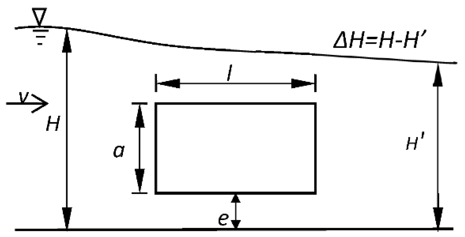
The hydrodynamic parameter schemes are detailed in Figure 1. In this figure, l is the length of the orifice-weir, m; a is the height of the orifice-weir, m; H’ is the downstream water depth, m; and ΔH is the water level difference, m, ΔH = H − H’.
The critical conditions for discriminating orifice flow and weir flow are obtained by using the following formulas for a broad-crested weir:
- (a)
- Orifice flow: β = 1, γ = 0.5;
- (b)
- Combined orifice-weir flow: e + a < H, e > 0 and β + γ = 1.5;
- (c)
- Weir flow: β = 0; γ = 1.5.
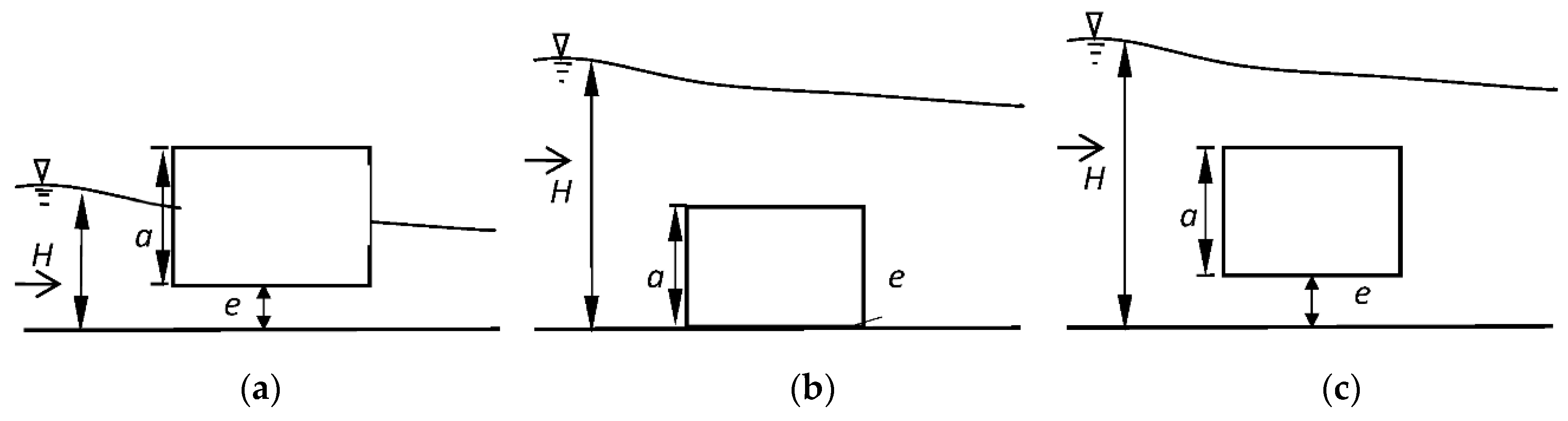
Figure 2a shows the orifice flow state. The upstream water level does not exceed the structure but is greater than the orifice height, that is, e ≤ H ≤ e + a. Therefore, the equation for flow is β = 1, γ = 0.5; . In the orifice-weir flow, the critical condition of the orifice pattern changes to H = e + a, which means (e + a)/H = 1; the critical condition between the orifice flow and the combined orifice-weir flow is used to define the index β, thus, the function β = (e + a)/H is obtained.
Figure 2b shows the weir flow situation, and Equation (2), , is the discharge formula for weir flow. If the e is very small, and the upstream level H >> e + a; thus, the discharge through the orifice can be approximately neglected and the flow pattern is similar to weir flow.
To obtain the pattern of combined orifice-weir flow, the upstream depth must exceed the structure. In Figure 2c, the combined orifice-weir flow is e + a < H, e > 0. To ensure that the formulae have dimensional uniformity, β + γ = 1.5, and the function (e + a)/H is used to define the index β. The discharge formula for combined orifice-weir flow is deduced through two critical conditions of orifice flow and weir flow, and it can only be used in the following condition:under submerged flow.
Indices β and γ are written as a function of e, a and H:
The discharge formula for combined orifice-weir flow is deduced through two critical conditions of orifice flow and weir flow under the combined flow. Combining Equations (2) and (3), the following discharge formula for combined orifice-weir flow is obtained:
Fluid characteristics and channel properties are the parameters affecting the discharge coefficient. Therefore, in Equation (4), m is related to ΔH ([L]), e ([L]), a ([L]), l ([L]), H ([L]), g ([L/T2]), the mass density of the fluid ρ (FT2/L4), the dynamic viscosity of the fluid ([FT/L2]), and the surface tension ([F/L]). The following equation for the discharge coefficient is obtained:
in which are fluid characteristics. H, g, and are selected as the basic parameters. Based on the π theorem, the following dimensionless Pi-groups are proposed: π1 = e/H, π2 = a/H, π3 = l/H, π4 = ΔH/H, π5 = Re, and π6 = We. For the discharge rate, the viscous effects represented as π5 = Re and the effect of surface tension represented as π6 = We can be neglected. Therefore, the effects of viscosity and surface tension are negligible [9,11,22]. On the basis of the Buckingham theorem and according to Barenbaltt and Di Stefano, “in some cases, it turns out to be convenient to choose new similarity parameters” [23,24]. Consequently, π groups can be combined to obtain new similarity terms. In general, the shape of the orifice-weir structure (l/a) and the height ratio of the orifice to orifice-weir (e/a) are the relevant parameters that determine the position and properties of structures. By combining the derived nondimensional groups, the dimensionless parameters were rearranged logically to yield and these relevant parameters are obtained:
Let Π2 = π1/π2 = (e/H)/(a/H) = e/a and Π3 = π3/π2 = (l/H)/(a/H) = l/a. Thus, a new non-dimensional equation for m can be written as follows:
Equation (6) is applied to H > e + a and e > 0, it is used for combined orifice-weir flow under submerged flow conditions and is highly convenient for the calculation of the flow coefficient.
2.2. Experimental Facility
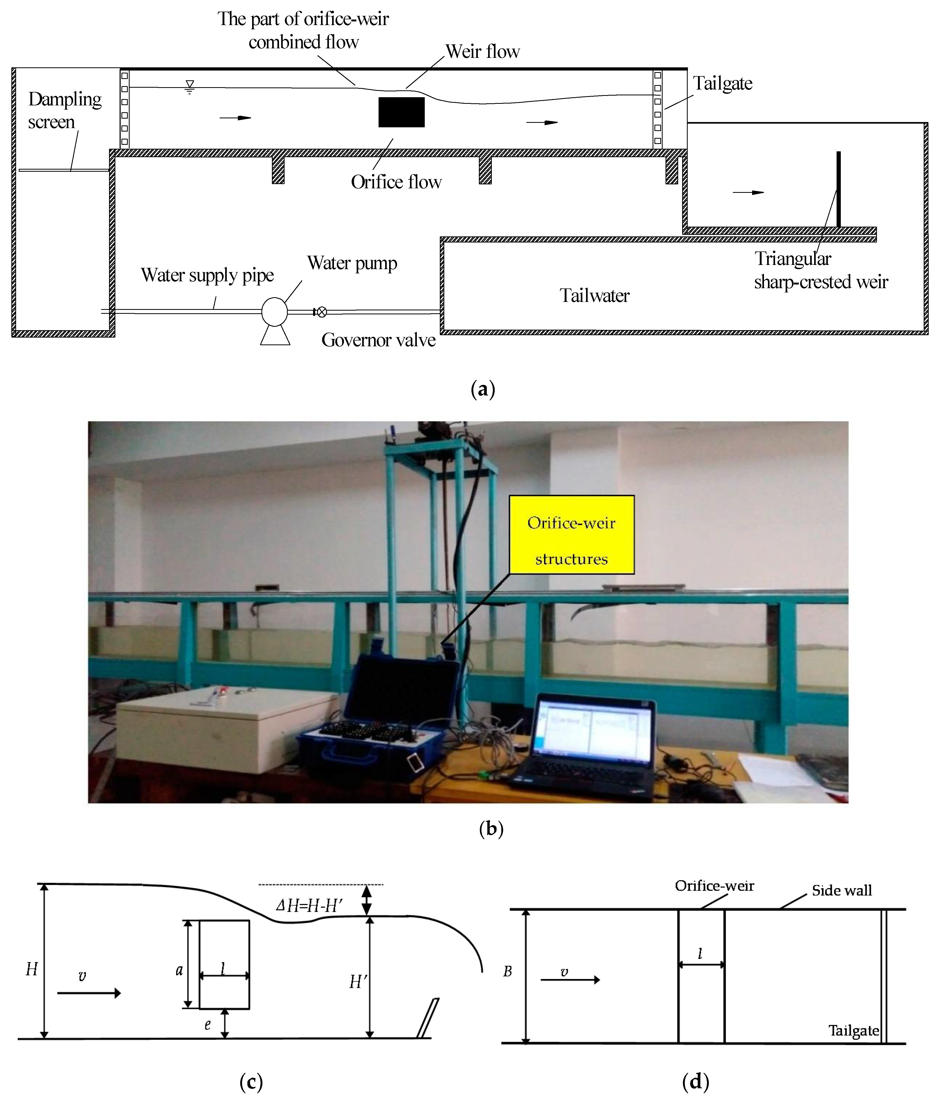
The experiments were carried out in a flume at the Hydraulic Laboratory, Hohai University. These experiments were conducted in a rectangular channel that was 0.5 m deep, 0.3 m wide, and 10 m long. The channel was supported by a platform 1.0 m above the floor and the slope of the flume was 0. The experimental rig was a self-circulation system, composed of a water pump, control valve, damping screen, glass flume, tailgate, triangular sharp-crested weir, and tailwater. Figure 3 shows the layout and a sketch of the experimental rig. A damping screen was installed upstream of the flume to calm the flow. The testing area for the combined orifice-weir flow was in the center of the flume. The width of the orifice-weir structure is the same as the width of the channel; that is, the contraction coefficient is 1. The water flows through the upper and lower parts of the structure to the downstream area. The tailgate was located at the end to regulate the water level. The water supply to the flume was provided through the supply pipe with a valve that controlled the flow. The discharge was measured at a triangular sharp-crested weir at the end of the flume. The water level was measured upstream and downstream in all experimental runs by a point gauge with an accuracy of ±0.01 cm. The experiments were conducted under conditions of steady flow and submerged flow. The tailgate affected the upstream depth and consequent discharge, and the typical velocities were obtained by particle image velocimetry (PIV). The flow characteristics around the orifice-weir structure were measured along the longitudinal section.
2.3. Experimental Tests
The contributing parameters were adjusted in the experiments on combined orifice-weir flow to evaluate the variation in the discharge coefficient. Experiments were conducted under submerged flow conditions for four orifice-weir distances a = 5, 10, 15, and 20 cm, five orifice heights e = 2, 5, 10, 15, and 20 cm and four inflow unit discharge rates q = 0.05, 0.06, 0.07, and 0.08 m2/s. The length of the orifice-weir was l = 10, 20, 30, and 40 cm, and the width of the orifice-weir was B = 30 cm, perpendicular to the flume. A total of 284 test runs were performed. All the experimental data are listed in Appendix A.
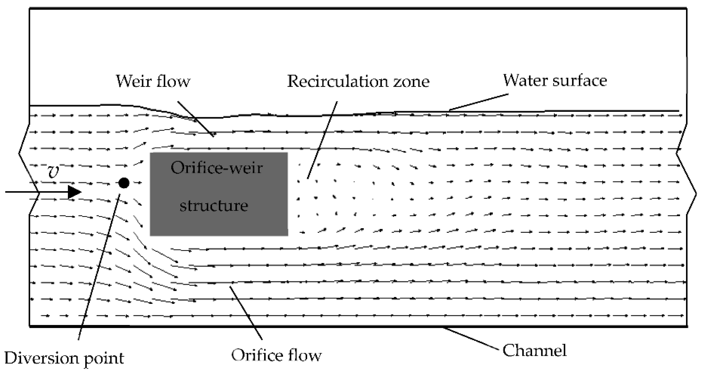
Figure 4 shows a schematic diagram of the flow. A diversion point exists near the center of the upstream surface along the longitudinal section; at this point, the velocity perpendicular to the flow direction is zero. The flow from the upstream region passing over and under the orifice-weir structure separated at this diversion point, the flow on the top of the structure becomes the weir flow, and the flow beneath becomes a pressurized orifice flow. The vertical position of the point was measured. The water surface profile drops slightly before the upstream region of the weir crest and then declines sharply along the orifice-weir structure. The presence of the orifice-weir structure creates a recirculation zone in the downstream region. The orifice flow discharge is affected by the recirculation zone due to a reduction in the kinetic energy; thus, the discharge capacity of the orifice-weir is decreased.
3. Results and Discussions
3.1. Effects of Contributing Parameters on m
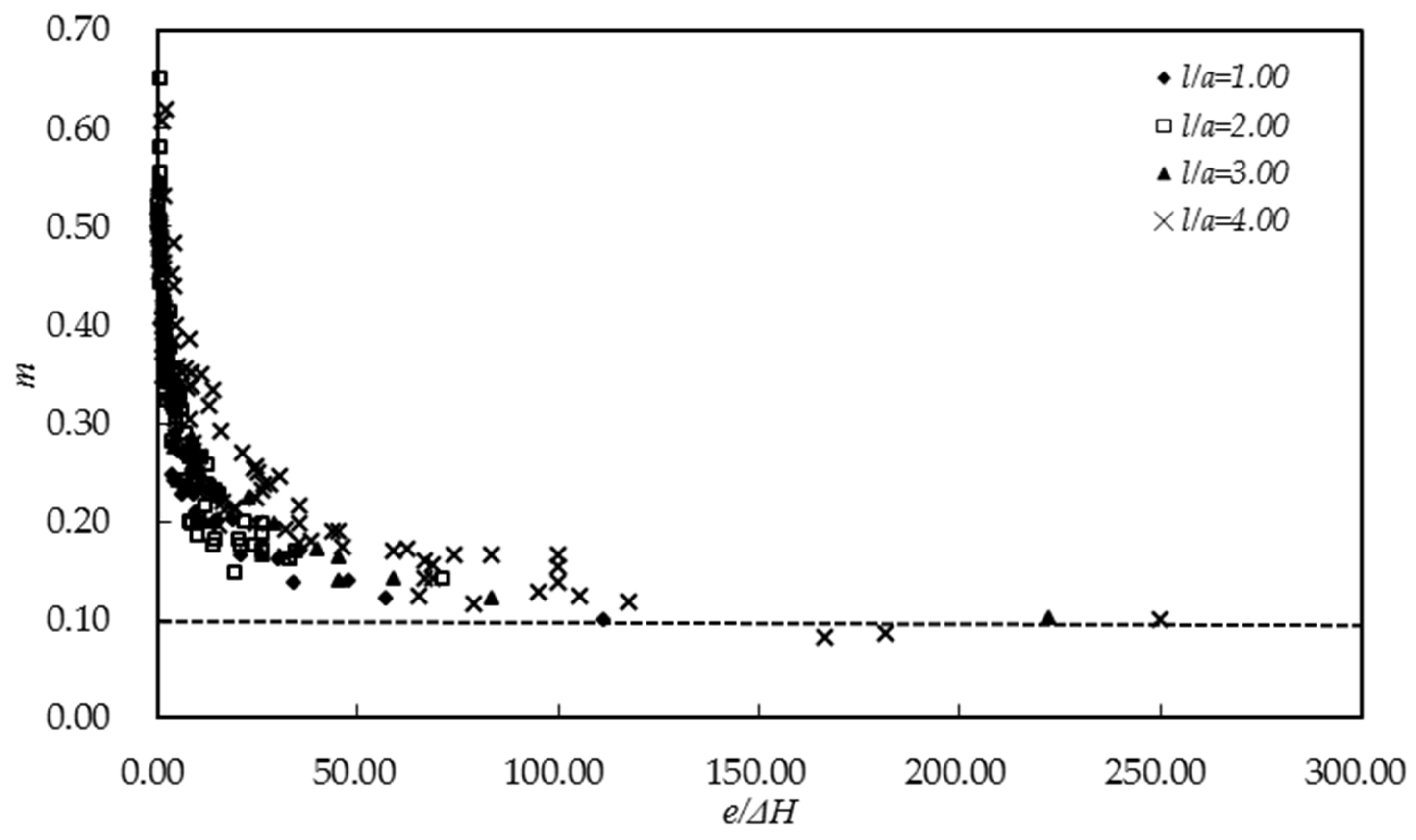
The m values are plotted against e/ΔH for different values of l/a in Figure 5. In particular, the combined orifice-weir flow with e/ΔH < 10 results in higher m values. Compared with a classic broad-crested weir and a waterways experiment station (WES) weir, which are commonly used in water conservancy projects as discharge weirs, the discharge area of the combined orifice-weir is larger for a given weir height under submerged conditions. A negative power-function relationship exists between m and e/ΔH, and the values of l/a have little effect on the m values. The value of m decreases significantly with a slight increase in e/ΔH values if e/ΔH < 100. The effect of small ΔH values on m is evident. A larger ΔH value is required to obtain a high m value in actual situations. As shown in Figure 4, the range of m decreases as the value of e/ΔH increases, and the value of m gradually stabilizes at high values of e/ΔH. If m is close to 0.1, the discharge coefficient values tend to plot along a horizontal line, which means that e/ΔH has no significant effect on m.
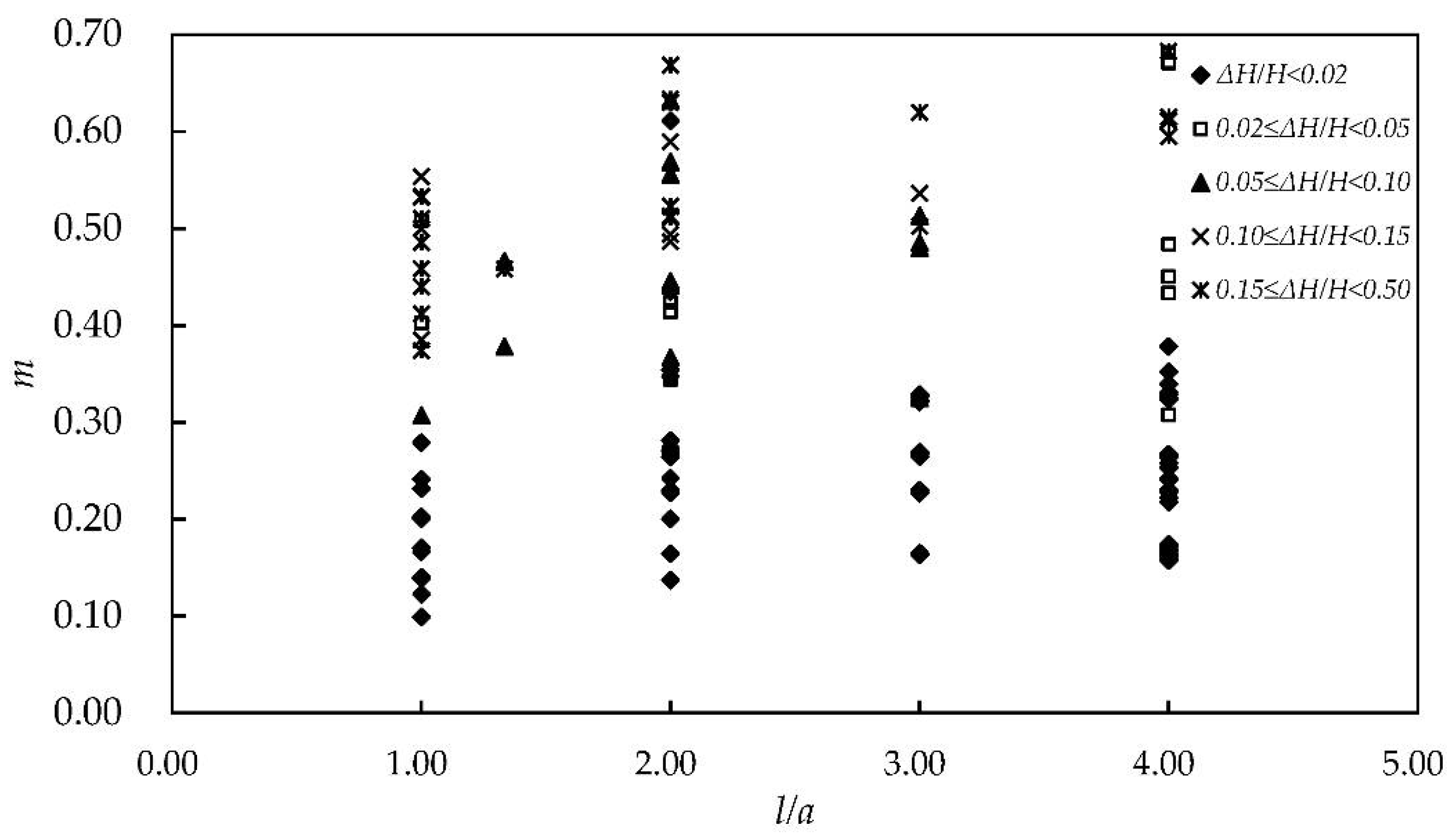
The relationships between m and l/a for different ΔH/H are compared in Figure 6. The flow in all the experimental tests was subcritical to ensure that the flow state is combined orifice-weir flow. Five different shapes of orifice-weir structures were used. Changes to the length of the orifice-weir structure did not result in significant changes in the position of the diversion point and it remained upstream of the structure and at a height approximately equivalent to the center of the structure. Thus, the structure length has no significant effect on the proportion of orifice flow to the weir flow. In all cases, as the value of l/a increases, the value of m does not change significantly under different ΔH/H values. Similarly, the ratio of weir flow to orifice flow did not change significantly with the changes in the orifice-weir distance. Thus, the effect of different values of l/a on m is not obvious.
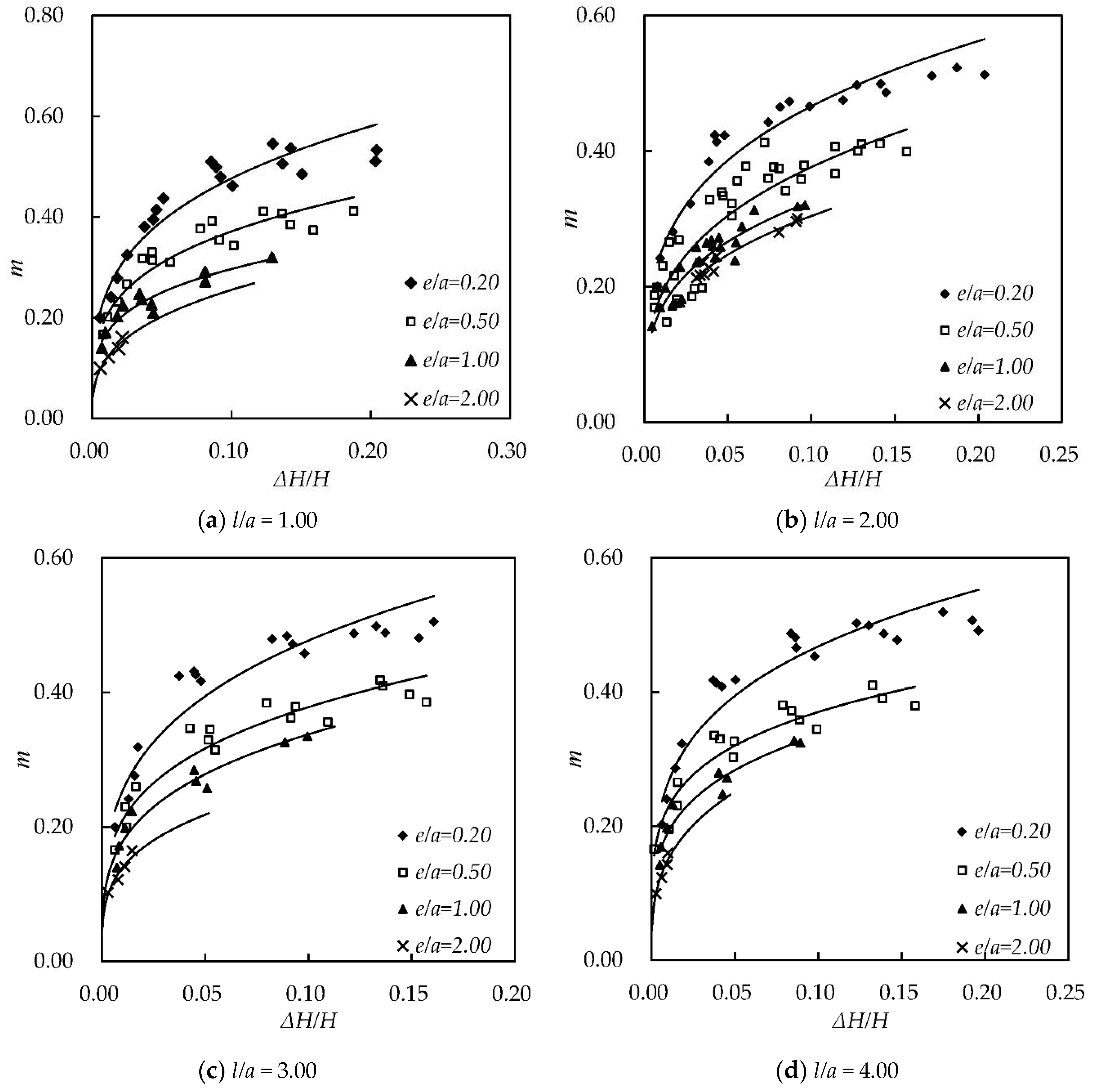
The relationships between m values and ΔH/H values for different values of the ratios e/a and l/a are compared in Figure 7. A greater value of ΔH/H significantly increases m for the same e/a, and with a smaller ΔH/H, the gradient of m becomes larger. The change in m becomes obvious if ΔH/H approaches 0. A larger ΔH is required to obtain a high value of m in actual situations, which is similar to previously discussed trends. There is a limiting effect on the discharge capacity and this limited discharge capacity produces a higher water level upstream of the orifice-weir region. A high downstream water depth results in a small water level and high submergence, leading to a lower discharge capacity. ΔH/H exhibits a nonlinear power function relationship in all cases. The effect of e/a on m is different for the same ΔH/H value among the orifice-weir lengths. For the same value of ΔH/H, a lower value of e/a results in a higher value of m. Additionally, a comparison of the values of m for different values of l/a reveals that different l/a values have little effect on the range of m values.
3.2. Empirical Discharge Formula and Sensitivity Analysis
According to Equation (6), the following dimensionless factors are related to compute the value of m for combined orifice-weir flow: Based on the ordinary least squares method, statistical regression analysis via the nonlinear regression (NLR) and multiple linear regression (MLR) methods was used to derive m. To obtain the optimal model and to compare the sensitivity of each parameter, five models were constructed by using different sets of parameters. The five models with different parameters are shown below:
Power function relationships exist between m and e/ΔH and between m and ΔH/H. Therefore, nonlinear least squares regression is used to obtain the new dimensionless basic parameter of the flow coefficient. To derive the formula for m, multivariable linear fitting for independent variables related to m is conducted. According to the models, the following relationships are provided to calculate m under submerged flow conditions:
where m is dimensionless and H, e, a, l, and ΔH are in meters. Equations (12)–(16) are valid for H > e + a; 0.758 H > e > 0.066 H, 1.0 ≤ ≤ 4.0, and 0.4 H > ΔH, and they are used in submerged conditions.
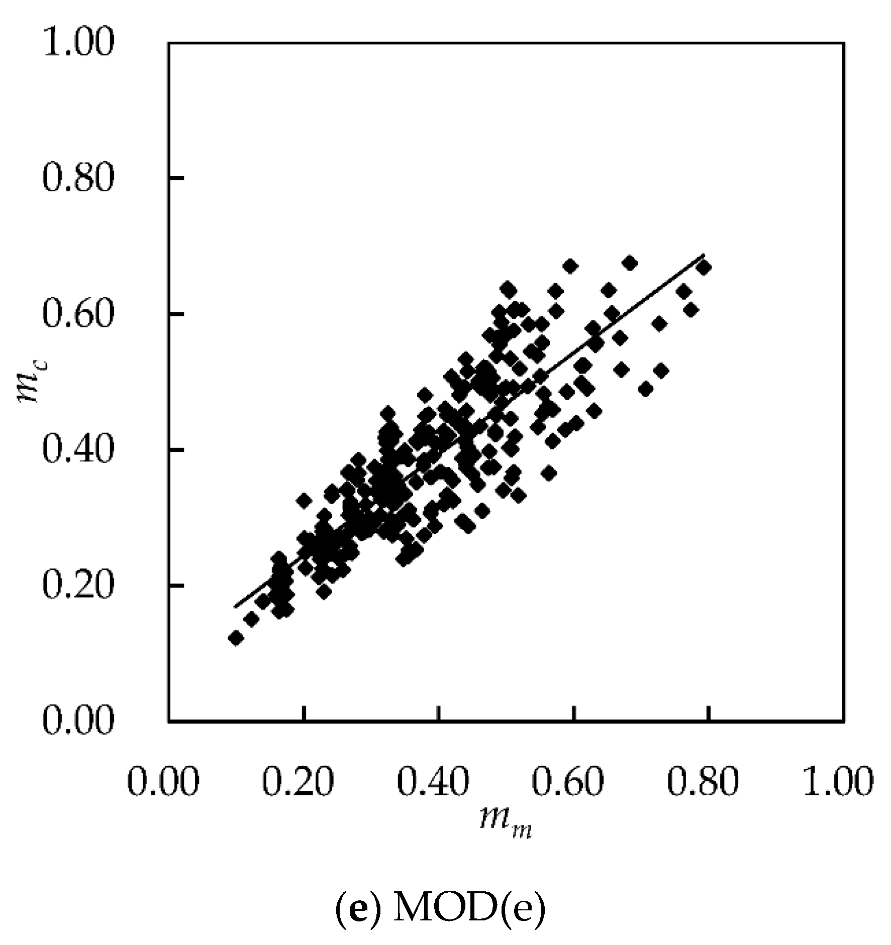
To evaluate the accuracy of the calculated discharge coefficient mcalculated (mc), comparisons between the measured discharge coefficient mmeasured (mm) and mc obtained by Equations (12)–(16) are shown in Table 1. The adjusted multiple correlation coefficient (AMCC), standard error of estimation (that is, the root mean square error, RMSE), and the mean absolute percent error (MAPE) are used. The AMCC indicates the goodness of fit of the m values and the RMSE evaluates the reliability of the data. The AMCC, RMSE, and MAPE are defined as follows:
where R2 is the coefficient of determination, K is the number of data sets, J is the number of dimensionless independent variable factors, and is the mean value of mm.
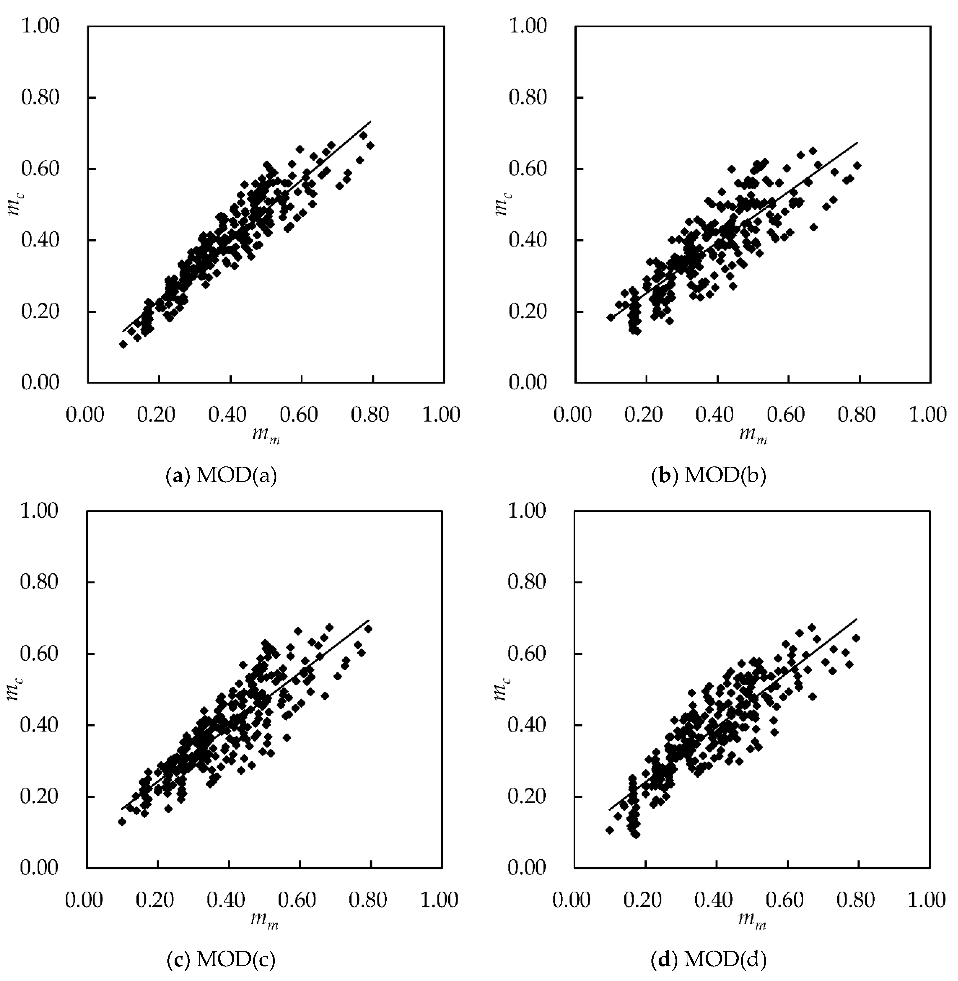
In Table 1, the values of the AMCC, RMSE, and MAPE are provided for the four models to compare the obtained m values. MOD(a) shows the best performance among the models, and the AMCC, RMSE, and MAPE values are 0.870, 0.053, and 0.058, respectively. The AMCC values of MOD(c) and MOD(d) are 0.756 and 0.762, respectively. The AMCC value of MOD(b) is 0.705, which corresponds to the lowest accuracy in the prediction of m. In addition, the indices in Table 1 are presented to highlight the sensitivity of the calculation to the parameters. The AMCC of MOD(d) is larger than that of MOD(b), which means that has a clear effect on the estimation of m, whereas l/a does not. In terms of sensitivity, the parameters can be arranged as follows:
Figure 8 shows comparisons between mc and mm for the four models. MOD(a) shows the best agreement with the experiments, whereas the accuracies of MOD(b) to MOD(e) are slightly lower than that of MOD(a). Thus, MOD(a) is recommended for calculating the discharge coefficient of combined orifice-weir flow under submerged flow conditions.
3.3. Verification and Error Analysis
MOD(a) includes all parameters and is used to calculate m. It is necessary to judge its applicability and fitting effect. An overall significance test is carried out by using the F-test. The 95% confidence interval is selected and the value of F is 247.18. The autocorrelation of MOD(a) is judged by the Durbin-Watson test (D − W) and the D − W value is 1.43, indicating that there is no autocorrelation. The Pearson correlation coefficients of the independent variables are low, which means they are not correlated. To eliminate instability, the variance expansion factor method is used to perform a multicollinearity diagnosis of MOD(a). The maximum value of VIF is 2.59; thus, there is no multicollinearity between variables. The definitions of the F-test, D-W test, and VIF are expressed as follows:
where et is the error term at time t and Ri2 is the coefficient of determination for different independent variables.
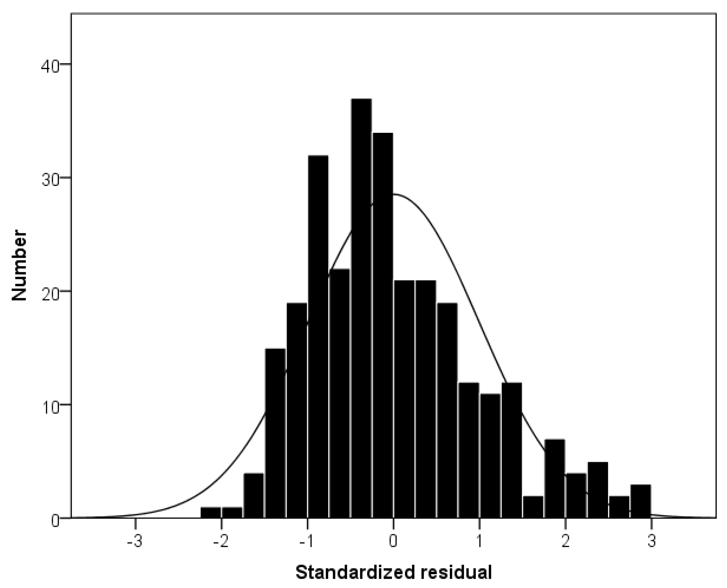
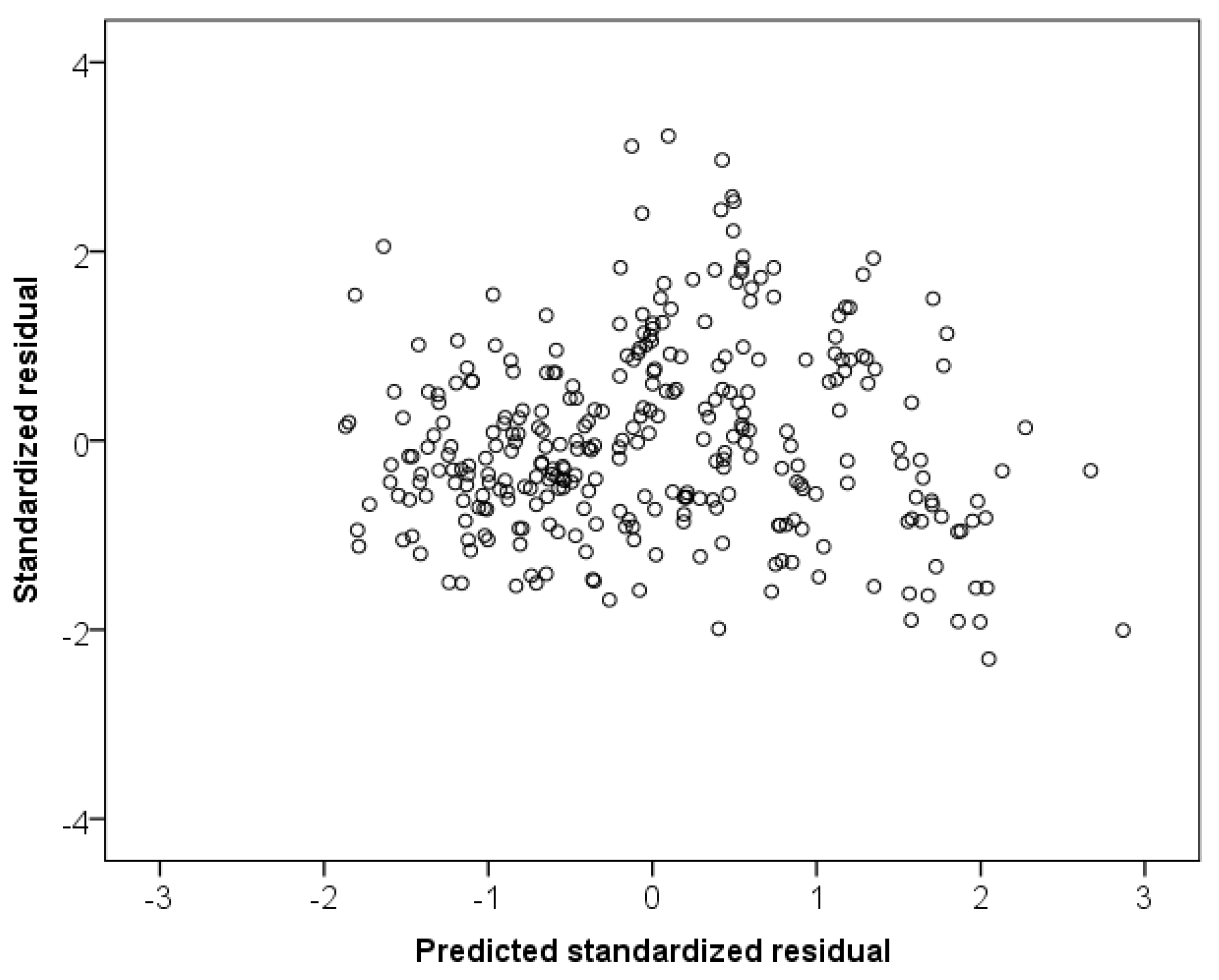
Figure 9 shows the distribution of the residuals of MOD(a) via a histogram of the residuals with a normal probability curve. As shown, the residuals present a normal distribution. The 95% distribution of the standardized residual data is between −2 and +2, which proves that the model assumptions are reasonable. Figure 10 shows a scatter plot of the standardized residual data.
MOD(a) is used to calculate the discharge capacity and shows a good applicability to the prediction of the discharge coefficient. Thus, the calculation formula for the discharge coefficient of the combined orifice-weir flow is obtained.
4. Conclusions
The discharge coefficient of combined orifice-weir flow is studied by means of theoretical analysis and physical model tests. A functional equation is derived by using dimensional analyses between combined orifice-weir flow discharge coefficients and the contributing parameters of upstream and downstream water level, orifice height, orifice-weir length, and orifice-weir height. Four dimensionless parameters, that is, the ratio of the water head to the upstream water level, the ratio of orifice height to orifice-weir height, the ratio of orifice height to the water head, and the ratio of the length to the height of the orifice-weir structure were obtained. The results demonstrate that if the ratio of orifice height to water level is small (that is, ≤100); the discharge coefficient increases significantly with decreases in this ratio; however, at larger ratios (that is, >100), the range of the coefficient approaches a straight line. Higher ratios of water level to upstream water level produce higher discharge coefficients and a lower ratio of orifice height to orifice-weir height results in a higher value of m. In contrast, the length-height ratio of the orifice-weir structure has little effect on the coefficient. In this study, nonlinear regression and multiple linear regression models are introduced to obtain five models to examine each of the dimensionless parameters. Statistical indices are used to evaluate the models and MOD(a) presents an acceptable degree of accuracy, with AMCC, RMSE, and MAPE values of 0.870, 0.053, and 0.058, respectively. In addition, the residuals of the equation for calculating the discharge coefficient of MOD(a) present a normal distribution. The results of MOD(a) agree with the experimental data and can thus provide a reference for estimating the discharge of combined orifice-weir flow. All the experiments were carried out in a subcritical flow state and the orifice-weir structure was submerged. Therefore, MOD(a) is valid for H > e + a; 0.758 H > e > 0.066 H, 1.0 ≤ ≤ 4.0, and 0.4 H > ΔH. However, this study does not consider the orifice-weir structure under supercritical flow conditions and the influence of such conditions on the discharge coefficient should be evaluated in the future.
Author Contributions
Z.-F.F. conceived and designed the experiments. Z.C. performed the experiments, analyzed the data and wrote the paper. W.-H.D. and Y.-J.C. improved the quality of the paper. The authors also thank the reviewers for their valuable comments, which significantly improved the quality of the paper.
Acknowledgments
The authors acknowledge the financial support provided by the National Key R&D Program of China (2016YFC0402501), the NSFC (51279048 and 51479071), the Fundamental Research Funds for the Central Universities (2016B40414), the 111 Project (B17015, B12032) and the Priority Academic Program Development of Jiangsu Higher Education Institutions (YS11001).
Conflicts of Interest
The authors declare no conflict of interest.
Abbreviations
The following symbols are used in this paper:
| a | orifice-weir distance |
| e | orifice height |
| Q | inflow discharge rate |
| l | length of the orifice-weir structure |
| B | width of the orifice-weir structure |
| H | upstream water depth |
| H’ | downstream water depth |
| ΔH | water level difference |
| v | average flow velocity |
| q | discharge per width of combined orifice-weir flow |
| g | gravitational acceleration |
| H0 | upstream water head; H0 = H + v2/2g |
| m | discharge coefficient of combined orifice-weir flow |
| Fr2 | Froude number: Fr2 = v2/gH |
| mc | calculated discharge coefficient |
| mm | measured discharge coefficient |
| R2 | coefficient of determination |
| AMCC | adjusted multiple correlation coefficient |
| RMSE | root mean square error |
| MAPE | the mean absolute percent error |
Appendix A

Table A1.
Experimental data for calculating the discharge coefficient of combined orifice-weir flow.
Table A1.
Experimental data for calculating the discharge coefficient of combined orifice-weir flow.
| Case | H/m | ΔH/m | q/(m2·s−1) | l/a | e/a | Case | H/m | ΔH/m | q/(m2·s−1) | l/a | e/a |
|---|---|---|---|---|---|---|---|---|---|---|---|
| 1 | 0.26 | 0.65 | 0.08 | 1.33 | 0.33 | 143 | 0.30 | 0.19 | 0.08 | 4.00 | 0.20 |
| 2 | 0.31 | 0.77 | 0.08 | 1.00 | 0.25 | 144 | 0.30 | 0.38 | 0.08 | 2.00 | 1.00 |
| 3 | 0.25 | 0.92 | 0.08 | 1.33 | 0.33 | 145 | 0.26 | 1.17 | 0.08 | 3.00 | 0.20 |
| 4 | 0.24 | 1.37 | 0.08 | 1.33 | 0.33 | 146 | 0.23 | 1.16 | 0.08 | 4.00 | 0.50 |
| 5 | 0.23 | 0.42 | 0.08 | 2.00 | 0.50 | 147 | 0.24 | 1.27 | 0.08 | 3.00 | 0.50 |
| 6 | 0.30 | 1.13 | 0.08 | 1.00 | 0.25 | 148 | 0.30 | 0.45 | 0.08 | 2.00 | 0.50 |
| 7 | 0.16 | 0.40 | 0.08 | 4.00 | 2.00 | 149 | 0.24 | 1.02 | 0.06 | 1.00 | 0.50 |
| 8 | 0.30 | 1.40 | 0.08 | 1.00 | 0.25 | 150 | 0.24 | 1.09 | 0.08 | 2.00 | 1.00 |
| 9 | 0.26 | 0.11 | 0.08 | 4.00 | 4.00 | 151 | 0.23 | 0.49 | 0.08 | 4.00 | 3.00 |
| 10 | 0.23 | 0.38 | 0.08 | 2.00 | 1.00 | 152 | 0.29 | 1.19 | 0.08 | 1.33 | 0.67 |
| 11 | 0.22 | 0.41 | 0.08 | 2.00 | 1.00 | 153 | 0.28 | 1.08 | 0.08 | 2.00 | 0.20 |
| 12 | 0.22 | 0.49 | 0.08 | 2.00 | 1.00 | 154 | 0.30 | 0.22 | 0.08 | 3.00 | 1.00 |
| 13 | 0.22 | 1.10 | 0.08 | 4.00 | 0.20 | 155 | 0.21 | 4.30 | 0.06 | 1.00 | 0.20 |
| 14 | 0.18 | 0.31 | 0.08 | 4.00 | 2.00 | 156 | 0.23 | 1.37 | 0.08 | 2.00 | 1.00 |
| 15 | 0.21 | 1.12 | 0.08 | 2.00 | 0.50 | 157 | 0.25 | 2.06 | 0.08 | 3.00 | 0.20 |
| 16 | 0.27 | 0.12 | 0.08 | 4.00 | 4.00 | 158 | 0.30 | 0.39 | 0.08 | 3.00 | 0.20 |
| 17 | 0.22 | 0.48 | 0.08 | 2.00 | 1.00 | 159 | 0.20 | 3.04 | 0.05 | 1.00 | 0.20 |
| 18 | 0.18 | 0.40 | 0.08 | 4.00 | 2.00 | 160 | 0.22 | 1.97 | 0.08 | 4.00 | 0.50 |
| 19 | 0.28 | 0.77 | 0.08 | 1.33 | 0.33 | 161 | 0.30 | 0.66 | 0.08 | 1.00 | 1.00 |
| 20 | 0.20 | 3.13 | 0.08 | 3.00 | 0.20 | 162 | 0.23 | 3.03 | 0.08 | 4.00 | 0.20 |
| 21 | 0.20 | 0.28 | 0.08 | 4.00 | 2.00 | 163 | 0.21 | 2.04 | 0.05 | 2.00 | 0.20 |
| 22 | 0.24 | 0.88 | 0.08 | 3.00 | 0.20 | 164 | 0.30 | 0.29 | 0.08 | 4.00 | 4.00 |
| 23 | 0.20 | 1.89 | 0.08 | 2.00 | 0.50 | 165 | 0.30 | 0.28 | 0.06 | 1.00 | 1.00 |
| 24 | 0.23 | 0.89 | 0.08 | 2.00 | 0.50 | 166 | 0.26 | 1.94 | 0.08 | 2.00 | 0.20 |
| 25 | 0.14 | 2.39 | 0.08 | 4.00 | 1.00 | 167 | 0.22 | 0.60 | 0.08 | 4.00 | 3.00 |
| 26 | 0.21 | 2.05 | 0.08 | 4.00 | 0.20 | 168 | 0.27 | 1.00 | 0.08 | 2.00 | 0.50 |
| 27 | 0.16 | 1.23 | 0.08 | 4.00 | 1.00 | 169 | 0.30 | 0.25 | 0.08 | 3.00 | 1.00 |
| 28 | 0.16 | 1.38 | 0.08 | 4.00 | 1.00 | 170 | 0.24 | 2.93 | 0.08 | 1.00 | 0.50 |
| 29 | 0.30 | 0.14 | 0.08 | 2.00 | 1.00 | 171 | 0.21 | 2.93 | 0.08 | 4.00 | 0.50 |
| 30 | 0.19 | 2.98 | 0.08 | 2.00 | 0.50 | 172 | 0.30 | 0.75 | 0.08 | 1.00 | 0.50 |
| 31 | 0.28 | 0.93 | 0.08 | 1.33 | 0.33 | 173 | 0.23 | 2.97 | 0.07 | 2.00 | 0.20 |
| 32 | 0.22 | 1.23 | 0.08 | 2.00 | 0.50 | 174 | 0.25 | 1.04 | 0.08 | 2.00 | 1.00 |
| 33 | 0.17 | 5.14 | 0.08 | 2.00 | 0.50 | 175 | 0.23 | 1.16 | 0.08 | 3.00 | 1.00 |
| 34 | 0.18 | 0.59 | 0.08 | 4.00 | 1.00 | 176 | 0.30 | 0.54 | 0.07 | 1.00 | 0.20 |
| 35 | 0.23 | 0.19 | 0.08 | 4.00 | 3.00 | 177 | 0.31 | 0.18 | 0.05 | 1.00 | 2.00 |
| 36 | 0.21 | 0.23 | 0.08 | 4.00 | 3.00 | 178 | 0.23 | 2.17 | 0.08 | 3.00 | 0.50 |
| 37 | 0.21 | 3.02 | 0.08 | 4.00 | 0.20 | 179 | 0.22 | 0.59 | 0.08 | 4.00 | 3.00 |
| 38 | 0.23 | 1.08 | 0.08 | 2.00 | 0.50 | 180 | 0.22 | 2.09 | 0.08 | 2.00 | 1.00 |
| 39 | 0.21 | 1.66 | 0.08 | 2.00 | 0.50 | 181 | 0.23 | 0.53 | 0.08 | 4.00 | 3.00 |
| 40 | 0.20 | 0.31 | 0.08 | 4.00 | 2.00 | 182 | 0.22 | 3.08 | 0.06 | 2.00 | 0.20 |
| 41 | 0.21 | 1.18 | 0.08 | 3.00 | 0.50 | 183 | 0.20 | 4.03 | 0.05 | 1.00 | 0.20 |
| 42 | 0.28 | 1.20 | 0.08 | 1.33 | 0.33 | 184 | 0.23 | 4.00 | 0.08 | 4.00 | 0.20 |
| 43 | 0.17 | 0.75 | 0.08 | 4.00 | 2.00 | 185 | 0.28 | 0.96 | 0.08 | 1.00 | 1.00 |
| 44 | 0.22 | 2.06 | 0.08 | 3.00 | 0.20 | 186 | 0.30 | 0.17 | 0.05 | 1.00 | 0.20 |
| 45 | 0.20 | 3.95 | 0.08 | 4.00 | 0.20 | 187 | 0.25 | 0.42 | 0.08 | 4.00 | 3.00 |
| 46 | 0.21 | 2.35 | 0.08 | 2.00 | 0.50 | 188 | 0.30 | 0.53 | 0.07 | 1.00 | 1.00 |
| 47 | 0.30 | 0.19 | 0.08 | 2.00 | 0.50 | 189 | 0.30 | 1.07 | 0.08 | 1.33 | 0.67 |
| 48 | 0.19 | 0.47 | 0.08 | 4.00 | 2.00 | 190 | 0.30 | 0.28 | 0.08 | 4.00 | 0.20 |
| 49 | 0.18 | 0.63 | 0.08 | 4.00 | 2.00 | 191 | 0.22 | 3.06 | 0.07 | 1.00 | 0.50 |
| 50 | 0.25 | 0.18 | 0.08 | 4.00 | 3.00 | 192 | 0.31 | 0.08 | 0.08 | 4.00 | 2.00 |
| 51 | 0.19 | 0.59 | 0.08 | 4.00 | 1.00 | 193 | 0.23 | 0.56 | 0.08 | 4.00 | 3.00 |
| 52 | 0.21 | 2.04 | 0.08 | 2.00 | 0.50 | 194 | 0.30 | 0.34 | 0.08 | 3.00 | 0.50 |
| 53 | 0.19 | 3.01 | 0.08 | 3.00 | 0.50 | 195 | 0.25 | 3.01 | 0.08 | 2.00 | 0.20 |
| 54 | 0.27 | 1.61 | 0.08 | 1.33 | 0.33 | 196 | 0.30 | 0.15 | 0.08 | 4.00 | 1.00 |
| 55 | 0.20 | 2.20 | 0.08 | 3.00 | 0.50 | 197 | 0.22 | 3.05 | 0.08 | 3.00 | 0.50 |
| 56 | 0.30 | 0.19 | 0.08 | 2.00 | 0.50 | 198 | 0.31 | 5.57 | 0.08 | 1.00 | 0.25 |
| 57 | 0.20 | 0.41 | 0.08 | 4.00 | 2.00 | 199 | 0.21 | 3.99 | 0.06 | 2.00 | 0.20 |
| 58 | 0.22 | 1.60 | 0.08 | 2.00 | 0.50 | 200 | 0.20 | 2.93 | 0.05 | 2.00 | 0.20 |
| 59 | 0.24 | 1.00 | 0.08 | 4.00 | 0.20 | 201 | 0.27 | 0.99 | 0.08 | 4.00 | 0.20 |
| 60 | 0.28 | 1.33 | 0.08 | 1.33 | 0.33 | 202 | 0.22 | 1.22 | 0.05 | 1.00 | 0.50 |
| 61 | 0.26 | 0.20 | 0.08 | 4.00 | 4.00 | 203 | 0.30 | 0.33 | 0.06 | 1.00 | 0.50 |
| 62 | 0.29 | 0.17 | 0.08 | 4.00 | 4.00 | 204 | 0.30 | 1.28 | 0.08 | 1.33 | 0.67 |
| 63 | 0.21 | 1.13 | 0.08 | 2.00 | 1.00 | 205 | 0.27 | 0.43 | 0.08 | 4.00 | 4.00 |
| 64 | 0.27 | 1.86 | 0.08 | 1.33 | 0.33 | 206 | 0.30 | 0.48 | 0.08 | 3.00 | 0.20 |
| 65 | 0.20 | 2.88 | 0.08 | 2.00 | 0.50 | 207 | 0.25 | 2.08 | 0.08 | 4.00 | 0.20 |
| 66 | 0.22 | 3.01 | 0.08 | 3.00 | 0.20 | 208 | 0.30 | 0.36 | 0.08 | 3.00 | 0.50 |
| 67 | 0.24 | 2.08 | 0.08 | 1.00 | 0.20 | 209 | 0.23 | 3.94 | 0.07 | 2.00 | 0.20 |
| 68 | 0.22 | 1.94 | 0.08 | 4.00 | 0.20 | 210 | 0.22 | 2.01 | 0.06 | 1.00 | 0.50 |
| 69 | 0.27 | 0.21 | 0.08 | 4.00 | 4.00 | 211 | 0.25 | 1.03 | 0.08 | 4.00 | 0.50 |
| 70 | 0.30 | 0.23 | 0.08 | 2.00 | 0.50 | 212 | 0.30 | 0.56 | 0.07 | 1.00 | 0.50 |
| 71 | 0.25 | 1.26 | 0.07 | 1.00 | 0.20 | 213 | 0.26 | 2.38 | 0.08 | 1.33 | 0.67 |
| 72 | 0.30 | 0.05 | 0.08 | 4.00 | 0.50 | 214 | 0.30 | 0.17 | 0.08 | 4.00 | 1.00 |
| 73 | 0.16 | 2.61 | 0.08 | 4.00 | 1.00 | 215 | 0.30 | 0.63 | 0.08 | 2.00 | 0.50 |
| 74 | 0.16 | 2.28 | 0.08 | 4.00 | 1.00 | 216 | 0.31 | 0.66 | 0.08 | 1.00 | 2.00 |
| 75 | 0.23 | 2.08 | 0.07 | 1.00 | 0.20 | 217 | 0.26 | 1.90 | 0.08 | 2.00 | 0.50 |
| 76 | 0.31 | 0.09 | 0.08 | 3.00 | 2.00 | 218 | 0.26 | 1.12 | 0.08 | 3.00 | 0.50 |
| 77 | 0.22 | 0.33 | 0.08 | 4.00 | 3.00 | 219 | 0.27 | 5.23 | 0.08 | 1.33 | 0.33 |
| 78 | 0.23 | 1.42 | 0.08 | 2.00 | 0.50 | 220 | 0.24 | 1.60 | 0.08 | 2.00 | 1.00 |
| 79 | 0.25 | 1.13 | 0.08 | 3.00 | 0.20 | 221 | 0.27 | 0.94 | 0.07 | 1.00 | 1.00 |
| 80 | 0.24 | 1.09 | 0.06 | 1.00 | 0.20 | 222 | 0.30 | 0.41 | 0.06 | 1.00 | 0.20 |
| 81 | 0.18 | 1.13 | 0.08 | 4.00 | 1.00 | 223 | 0.30 | 0.53 | 0.08 | 3.00 | 0.20 |
| 82 | 0.30 | 0.19 | 0.08 | 3.00 | 0.20 | 224 | 0.21 | 2.11 | 0.08 | 3.00 | 1.00 |
| 83 | 0.22 | 0.34 | 0.08 | 4.00 | 3.00 | 225 | 0.20 | 4.03 | 0.05 | 2.00 | 0.20 |
| 84 | 0.26 | 3.20 | 0.08 | 1.33 | 0.33 | 226 | 0.30 | 0.34 | 0.08 | 3.00 | 1.00 |
| 85 | 0.22 | 1.08 | 0.08 | 4.00 | 0.50 | 227 | 0.30 | 0.83 | 0.08 | 2.00 | 0.20 |
| 86 | 0.24 | 1.13 | 0.08 | 2.00 | 0.50 | 228 | 0.25 | 3.05 | 0.08 | 3.00 | 0.20 |
| 87 | 0.24 | 3.06 | 0.08 | 1.00 | 0.20 | 229 | 0.23 | 1.97 | 0.08 | 4.00 | 0.50 |
| 88 | 0.20 | 2.02 | 0.08 | 4.00 | 0.50 | 230 | 0.27 | 2.19 | 0.08 | 1.33 | 0.67 |
| 89 | 0.24 | 0.76 | 0.08 | 2.00 | 1.00 | 231 | 0.23 | 0.99 | 0.08 | 4.00 | 1.00 |
| 90 | 0.29 | 0.20 | 0.08 | 4.00 | 4.00 | 232 | 0.30 | 0.35 | 0.06 | 1.00 | 2.00 |
| 91 | 0.24 | 0.79 | 0.08 | 2.00 | 1.00 | 233 | 0.27 | 1.08 | 0.08 | 2.00 | 1.00 |
| 92 | 0.19 | 3.05 | 0.08 | 4.00 | 0.50 | 234 | 0.24 | 3.08 | 0.08 | 2.00 | 0.50 |
| 93 | 0.23 | 1.19 | 0.08 | 3.00 | 0.50 | 235 | 0.30 | 0.24 | 0.08 | 3.00 | 2.00 |
| 94 | 0.22 | 0.97 | 0.05 | 1.00 | 0.20 | 236 | 0.21 | 3.00 | 0.06 | 1.00 | 0.50 |
| 95 | 0.22 | 3.06 | 0.08 | 4.00 | 0.20 | 237 | 0.22 | 2.96 | 0.08 | 4.00 | 0.50 |
| 96 | 0.22 | 2.04 | 0.06 | 1.00 | 0.20 | 238 | 0.30 | 0.21 | 0.05 | 1.00 | 1.00 |
| 97 | 0.31 | 3.13 | 0.08 | 1.00 | 0.25 | 239 | 0.25 | 1.13 | 0.08 | 3.00 | 1.00 |
| 98 | 0.23 | 1.04 | 0.08 | 2.00 | 1.00 | 240 | 0.30 | 0.65 | 0.08 | 2.00 | 1.00 |
| 99 | 0.24 | 2.12 | 0.08 | 3.00 | 0.20 | 241 | 0.20 | 3.82 | 0.06 | 1.00 | 0.50 |
| 100 | 0.15 | 3.36 | 0.08 | 4.00 | 1.00 | 242 | 0.30 | 0.52 | 0.07 | 2.00 | 0.20 |
| 101 | 0.23 | 3.21 | 0.07 | 1.00 | 0.20 | 243 | 0.30 | 0.43 | 0.08 | 4.00 | 0.20 |
| 102 | 0.23 | 0.99 | 0.06 | 2.00 | 0.20 | 244 | 0.21 | 2.09 | 0.05 | 1.00 | 0.50 |
| 103 | 0.28 | 1.05 | 0.08 | 1.00 | 0.20 | 245 | 0.25 | 3.03 | 0.08 | 4.00 | 0.20 |
| 104 | 0.22 | 1.22 | 0.08 | 2.00 | 1.00 | 246 | 0.30 | 0.29 | 0.06 | 2.00 | 0.20 |
| 105 | 0.18 | 7.60 | 0.08 | 2.00 | 0.50 | 247 | 0.25 | 2.06 | 0.08 | 1.00 | 1.00 |
| 106 | 0.30 | 0.29 | 0.08 | 2.00 | 1.00 | 248 | 0.25 | 3.97 | 0.08 | 3.00 | 0.20 |
| 107 | 0.23 | 1.87 | 0.08 | 2.00 | 0.50 | 249 | 0.24 | 0.60 | 0.08 | 4.00 | 1.00 |
| 108 | 0.22 | 4.14 | 0.08 | 4.00 | 0.20 | 250 | 0.25 | 2.00 | 0.08 | 3.00 | 0.50 |
| 109 | 0.27 | 2.55 | 0.08 | 1.33 | 0.33 | 251 | 0.23 | 3.17 | 0.08 | 3.00 | 0.50 |
| 110 | 0.30 | 4.33 | 0.08 | 1.00 | 0.25 | 252 | 0.24 | 2.18 | 0.08 | 2.00 | 1.00 |
| 111 | 0.22 | 2.01 | 0.08 | 3.00 | 0.50 | 253 | 0.30 | 0.50 | 0.08 | 3.00 | 0.50 |
| 112 | 0.30 | 0.34 | 0.08 | 2.00 | 0.50 | 254 | 0.30 | 0.44 | 0.08 | 3.00 | 1.00 |
| 113 | 0.24 | 1.00 | 0.08 | 2.00 | 1.00 | 255 | 0.30 | 0.24 | 0.05 | 1.00 | 0.50 |
| 114 | 0.22 | 1.04 | 0.05 | 2.00 | 0.20 | 256 | 0.20 | 3.12 | 0.05 | 1.00 | 0.50 |
| 115 | 0.25 | 0.97 | 0.08 | 4.00 | 0.20 | 257 | 0.24 | 3.07 | 0.08 | 1.00 | 1.00 |
| 116 | 0.30 | 0.19 | 0.08 | 3.00 | 0.50 | 258 | 0.26 | 1.15 | 0.08 | 3.00 | 1.00 |
| 117 | 0.22 | 2.86 | 0.08 | 2.00 | 0.50 | 259 | 0.22 | 1.93 | 0.08 | 4.00 | 1.00 |
| 118 | 0.27 | 0.99 | 0.08 | 1.00 | 0.50 | 260 | 0.30 | 0.32 | 0.08 | 4.00 | 0.50 |
| 119 | 0.23 | 0.39 | 0.08 | 4.00 | 3.00 | 261 | 0.32 | 7.36 | 0.08 | 1.00 | 0.25 |
| 120 | 0.25 | 1.08 | 0.07 | 1.00 | 0.50 | 262 | 0.30 | 0.55 | 0.08 | 4.00 | 0.20 |
| 121 | 0.25 | 1.09 | 0.07 | 2.00 | 0.20 | 263 | 0.25 | 1.06 | 0.06 | 1.00 | 1.00 |
| 122 | 0.28 | 0.27 | 0.08 | 4.00 | 4.00 | 264 | 0.31 | 0.59 | 0.07 | 1.00 | 2.00 |
| 123 | 0.19 | 7.21 | 0.08 | 2.00 | 0.50 | 265 | 0.30 | 0.28 | 0.08 | 4.00 | 1.00 |
| 124 | 0.21 | 3.11 | 0.08 | 3.00 | 0.50 | 266 | 0.27 | 1.01 | 0.08 | 4.00 | 0.50 |
| 125 | 0.22 | 2.95 | 0.06 | 1.00 | 0.20 | 267 | 0.28 | 2.57 | 0.08 | 1.33 | 0.67 |
| 126 | 0.25 | 0.79 | 0.08 | 2.00 | 1.00 | 268 | 0.24 | 1.11 | 0.08 | 4.00 | 1.00 |
| 127 | 0.21 | 2.08 | 0.05 | 1.00 | 0.20 | 269 | 0.24 | 1.96 | 0.07 | 1.00 | 1.00 |
| 128 | 0.20 | 0.72 | 0.08 | 4.00 | 2.00 | 270 | 0.23 | 2.07 | 0.08 | 3.00 | 1.00 |
| 129 | 0.23 | 3.09 | 0.08 | 3.00 | 0.20 | 271 | 0.30 | 0.60 | 0.08 | 2.00 | 2.00 |
| 130 | 0.24 | 2.04 | 0.08 | 4.00 | 0.20 | 272 | 0.31 | 0.34 | 0.08 | 3.00 | 2.00 |
| 131 | 0.29 | 0.97 | 0.08 | 1.33 | 0.67 | 273 | 0.25 | 1.98 | 0.08 | 4.00 | 0.50 |
| 132 | 0.29 | 0.92 | 0.08 | 1.33 | 0.67 | 274 | 0.30 | 0.19 | 0.08 | 4.00 | 2.00 |
| 133 | 0.18 | 1.25 | 0.08 | 4.00 | 2.00 | 275 | 0.30 | 0.38 | 0.08 | 4.00 | 1.00 |
| 134 | 0.30 | 0.75 | 0.08 | 1.00 | 0.20 | 276 | 0.30 | 0.47 | 0.08 | 4.00 | 0.50 |
| 135 | 0.20 | 0.88 | 0.08 | 4.00 | 2.00 | 277 | 0.30 | 0.47 | 0.08 | 4.00 | 0.50 |
| 136 | 0.25 | 2.12 | 0.08 | 1.00 | 0.50 | 278 | 0.23 | 1.01 | 0.05 | 1.00 | 1.00 |
| 137 | 0.22 | 1.94 | 0.06 | 2.00 | 0.20 | 279 | 0.30 | 0.24 | 0.05 | 2.00 | 0.20 |
| 138 | 0.23 | 1.82 | 0.07 | 1.00 | 0.50 | 280 | 0.26 | 1.06 | 0.08 | 4.00 | 1.00 |
| 139 | 0.25 | 0.93 | 0.08 | 2.00 | 1.00 | 281 | 0.30 | 0.44 | 0.08 | 3.00 | 2.00 |
| 140 | 0.27 | 0.32 | 0.08 | 4.00 | 4.00 | 282 | 0.24 | 2.01 | 0.08 | 4.00 | 1.00 |
| 141 | 0.29 | 1.04 | 0.08 | 1.33 | 0.67 | 283 | 0.31 | 0.29 | 0.08 | 4.00 | 2.00 |
| 142 | 0.24 | 1.94 | 0.07 | 2.00 | 0.20 | 284 | 0.31 | 0.30 | 0.08 | 4.00 | 2.00 |
References
- Fu, Z.F.; Yin, X.J.; Gu, X.F. Hydraulic Characteristics of Floating Sluices Subsiding and Buoying in Flowing water. Adv. Sci. Technol. Water Resour. 2014, 34, 24–27. [Google Scholar]
- Cui, Z.; Fu, Z.F.; Chen, Y.J.; Wang, S.; Ma, G.G.; Jiang, W. Explore the Hydrodynamic Force on the Surface of Floating Structure in Finite Flowing Water. In Proceedings of the 37th IAHR World Congress, Kuala Lumpur, Malaysia, 13–18 August 2017. [Google Scholar]
- Cui, Z.; Fu, Z.; Dai, W.; Lai, Z. Submerged Fixed Floating Structure under the Action of Surface Current. Water 2018, 10, 102. [Google Scholar] [CrossRef]
- El-Belasy, A.M. Developing Formulae for combined weir and orifice(case study: EL-Fayoum weirs). Alex. Eng. J. 2013, 763–768. [Google Scholar] [CrossRef]
- Cimorelli, L.; Cozzolino, L.; Della Morte, R.; Pianese, D. Analytical solutions of the linearized parabolic wave accounting for downstream boundary condition and uniform lateral inflows. Adv. Water Resour. 2014, 63, 57–76. [Google Scholar] [CrossRef]
- Cozzolino, L.; Morte, R.D.; Cimorelli, L.; Covelli, C.; Pianese, D. A Broad-crested Weir Boundary Condition in Finite Volume Shallow-water Numerical Models. Procedia Eng. 2014, 70, 353–362. [Google Scholar] [CrossRef]
- Cozzolino, L.; Cimorelli, L.; Covelli, C.; Della Morte, R.; Pianese, D. The analytic solution of the Shallow-Water Equations with partially open sluice-gates: The dam-break problem. Adv. Water Resour. 2015, 80, 90–102. [Google Scholar] [CrossRef]
- Alhamid, A.A. Analysis and formulation of flow through combined V-notch-gate-device. J. Hydraul. Res. 1999, 37, 697–705. [Google Scholar] [CrossRef]
- Negm, A.M.; Al-Brahim, A.M.; Alhamid, A.A. Combined-free flow over weirs and below gates. J. Hydraul. Res. 2002, 3, 359–365. [Google Scholar] [CrossRef]
- Xu, G.; Wang, Y.H. Discharge Calculation of Hydraulic Automatic Flap Gate. Zhejiang Hydrotech. 2014, 62–65. [Google Scholar]
- Altan-Sakarya, A.B.; Kökpınar, M.A. Computation of discharge for simultaneous flow over weirs and below gates (H-weirs). Flow Meas. Instrum. 2013, 29, 32–38. [Google Scholar] [CrossRef]
- Negm, A.M.; Al-Brahim, A.M.; Alhamid, A.A.; Sakarya, B.A.; Aydin, I.; Ger, A.M. Combined free flow over weirs and below gates. J. Hydraul. Res. 2004, 5, 559–562. [Google Scholar] [CrossRef]
- Negm, A.M.; Ezzeldin, M.; Attia, M.I. Characteristics of simultaneous flow over suppressed weirs and below submerged gates. Eng. Res. J. 1999, 65, 218–231. [Google Scholar]
- Negm, A.M.; Abdelaal, G.M.; Matin, A.M.; Alhamid, A.A. Discharge equation for free and submerged flow through combined weir. In Proceedings of the 3rd International Conference on Al-Azhar Engineering (AEIC-97), Cairo, Egypt, 19–22 December 1997; pp. 456–457. [Google Scholar]
- Negm, A.; M Abdel-Aal, G.; El-Saiad, A. Generalized discharge equation for proposed simultaneous flow structures. In Proceedings of the 6th Alahzer Engineering International Conference (AEIC-2000), Cairo, Egypt, 10–14 September 2000; pp. 247–257. [Google Scholar]
- Ferro, V. Simultaneous Flow over and under a Gate. J. Irrig. Drain. 2000, 126, 190–193. [Google Scholar] [CrossRef]
- AL-Saadi, A.K.I. Study Coefficient of Discharge for a Combined Free Flow over Weir. Euphrates J. Agric. Sci. 2013, 4, 26–35. [Google Scholar]
- Samani, J.M.V.; Mazaheri, M. Combined flow over weir and under gate. J. Hydraul. Eng. 2009, 135, 224–227. [Google Scholar] [CrossRef]
- Parsaie, A.; Azamathulla, H.M.; Haghiabi, A.H. Prediction of discharge coefficient of cylindrical weir gate using GMDH PSO. ISH J. Hydraul. Eng. 2018, 24, 116–123. [Google Scholar] [CrossRef]
- Alhamid, A.A.; Husain, D.; Negm, A.M. Discharge Equation for Simultaneous Flow over Rectangular Weirs and Below Inverted Triangular Weirs. Arab Gulf J. Sci. Res. 1996, 3, 595–607. [Google Scholar]
- Guo, W.; Pei, G.; Han, H. Hydraulics; China Water & Power Press: Beijing, China, 2005. [Google Scholar]
- Severi, A.; Masoudian, M.; Kordi, E.; Roettcher, K.; Roettcher, K. Discharge coefficient of combined free over under flow on a cylindrical weir gate. J. Hydraul. Eng. 2015, 1, 42–52. [Google Scholar] [CrossRef]
- Di Stefano, C.; Ferro, V. Stage—Discharge Relationship for an Upstream Inclined Grid with Transversal Bars. J. Irrig. Drain. Eng. 2016, 142, 07016008. [Google Scholar] [CrossRef]
- Barenblatt, G.I. Dimensional Analysis; Gordon & Breach, Science Publishers: Amsterdam, The Netherlands, 1987. [Google Scholar]
Figure 1.
The parameters of combined orifice-weir flow.

Figure 2.
The sketches of different flow states: (a) orifice flow; (b) weir flow; (c) combined orifice-weir flow.
Figure 2.
The sketches of different flow states: (a) orifice flow; (b) weir flow; (c) combined orifice-weir flow.

Figure 3.
The layout and the sketch of the experimental rig: (a) the experimental rig; (b) the main experimental rig area; (c) the front view; (d) the plan view.
Figure 3.
The layout and the sketch of the experimental rig: (a) the experimental rig; (b) the main experimental rig area; (c) the front view; (d) the plan view.

Figure 4.
The schematic diagram of the flow.

Figure 5.
The plot of m versus e/ΔH for l/a values.

Figure 6.
m as a function of l/a for different ΔH/H values.

Figure 7.
m as a function of ΔH/H for different l/a values.

Figure 8.
The comparisons between mc and mm.


Figure 9.
The distribution of the standardized residual data (mean = 0, standard deviation = 0.994, N = 284).
Figure 9.
The distribution of the standardized residual data (mean = 0, standard deviation = 0.994, N = 284).

Figure 10.
The scatter plots of the standardized residual data.

Table 1.
The AMCC, RMSE, and MAPE values for the five models.
| Indexes | MOD(a) | MOD(b) | MOD(c) | MOD(d) | MOD(e) |
|---|---|---|---|---|---|
| AMCC | 0.870 | 0.705 | 0.756 | 0.762 | 0.739 |
| RMSE | 0.053 | 0.076 | 0.069 | 0.068 | 0.072 |
| MAPE | 0.058 | 0.103 | 0.059 | 0.282 | 0.103 |
© 2018 by the authors. Licensee MDPI, Basel, Switzerland. This article is an open access article distributed under the terms and conditions of the Creative Commons Attribution (CC BY) license (http://creativecommons.org/licenses/by/4.0/).
Share and Cite
MDPI and ACS Style
Fu, Z.-F.; Cui, Z.; Dai, W.-H.; Chen, Y.-J. Discharge Coefficient of Combined Orifice-Weir Flow. Water 2018, 10, 699. https://doi.org/10.3390/w10060699
AMA Style
Fu Z-F, Cui Z, Dai W-H, Chen Y-J. Discharge Coefficient of Combined Orifice-Weir Flow. Water. 2018; 10(6):699. https://doi.org/10.3390/w10060699
Chicago/Turabian StyleFu, Zong-Fu, Zhen Cui, Wen-Hong Dai, and Yue-Jun Chen. 2018. "Discharge Coefficient of Combined Orifice-Weir Flow" Water 10, no. 6: 699. https://doi.org/10.3390/w10060699
Note that from the first issue of 2016, this journal uses article numbers instead of page numbers. See further details here.