Hydrologic Modeling of Three Sub-Basins in the Kenai River Watershed, Alaska, USA


1
Alaska Department of Transportation and Public Facilities, 6860 Glacier Highway, Juneau, AK 99801, USA
2
Department of Civil and Environmental Engineering, University of Alaska Fairbanks, 505 N. Chandalar Dr., Fairbanks, AK 99775, USA
*
Author to whom correspondence should be addressed.
Water 2018, 10(6), 691; https://doi.org/10.3390/w10060691
Submission received: 3 March 2018
/
Revised: 18 May 2018
/
Accepted: 23 May 2018
/
Published: 25 May 2018
(This article belongs to the Section Hydrology)
Abstract
:Streams in the Kenai River watershed are characterized by a fish-rich environment. The commercial fishing industry and recreational users compete for the fish in these streams, and resource managers strive to balance both groups’ needs while maintaining the sustainability of the resource. The ability to estimate future river conditions could help preserve the resource and a strong economy on the Kenai Peninsula. This research used the U.S. Army Corps of Engineers Hydrological Modeling System, which transforms rainfall to river discharge. The main goal was to define a set of parameters that were calibrated using an event-based condition of concurrent rainfall and discharge data. The model was calibrated and validated in three sub-basins located in different environmental settings (i.e., lowlands, mid, and high elevation).
1. Introduction
Residents of the Kenai Peninsula rely on rivers for both recreation and economic opportunities. Czarneski and Yaeger [1] describe it best in their Kenai River Center publication: “Healthy rivers, lakes and oceans are vital to healthy economies and good local standards of living, particularly on the Kenai Peninsula where so much of the economy and culture is centered on the water”.
The importance of the health of the water systems is recognized both by government agencies, and local industry. On its website, the Kenai River Sportfishing Association [2] discusses its goal to maintain the health of Alaskan fisheries. This goal can be achieved through the sustainable harvesting of resources, and protection of the habitat that the resources need to survive. An understanding of the watershed could provide a cornerstone for supporting the resources that exist in the area, and the economy which is served by those resources.
Though many agencies in the area study the basin, most of them focus on the water quality of anadromous streams in the watershed. The quality of the water in these streams is important, as are estimates of water temperature, low flows, and peak discharge values. However, the watershed is characterized by a scarcity of hydro-meteorological data. The goals of this research were to implement a hydrological model during the warm season (due to the lack of winter data), and to provide a set of calibrated parameters that can be used by other researchers to help answer questions related to the current and future hydrology of the Kenai River watershed, such as possible variability in discharge rates as the precipitation frequency and landscape change.
Three sub-basins in the Kenai River watershed were selected for hydrological modeling. These sub-basins represent the three hydrologic scenarios present in the watershed, i.e., low, middle, and steep gradients. Beaver Creek, located near Kenai, Alaska, is representative of a lowland, low-gradient wetlands stream. Russian River is a middle-gradient valley stream, and Ptarmigan Creek is a steep-gradient mountain stream. The Kenai River watershed and sub-basin areas, along with the selected sub-basins, are shown in Figure 1. The figures and tables in this article were adapted from Event Based Modeling Studying Three Sub-Basins in the Kenai River Watershed [3].
Communities on the Kenai Peninsula have survived thanks to the resources available in their region. Commercial and recreational fishing accounts for a large percentage of employment. A study of the local economy and of economic prospects on the Kenai Peninsula shows that 62% of gross earnings are from commercial fishing; about $72 million came solely from the harvest of salmon [4]. Though many regulations are currently in place to ensure the future of sport and commercial fisheries, most of the regulations are in place to protect the environmental quality of the water.
Factors that were not previously considered in the management of the watershed are becoming a concern—changes in precipitation patterns, for example. The Kenai Peninsula Borough states that the average total precipitation in the Kenai area is 48.9 cm [5]. Studies on the drying of the wetlands in the Kenai Peninsula Lowland and throughout south-central Alaska have been published [6]. Berg et al. reported that, since 1968, available water from precipitation has declined by 55% due to changes in evapotranspiration rates and precipitation amounts. All these potential changes could lead to changes in the availability and quality of salmon rearing habitat. With a heavy economic dependence on fisheries in the Kenai River watershed, a modeling tool is needed to help predict the effects of future precipitation, development, and landscape changes on the watershed.
2. Research Methods
The U.S. Army Corps of Engineers Hydrologic Engineering Center Hydrological Modeling System (HEC-HMS) was used as the modeling platform to accomplish the objective of this study. Because only sparse current and coinciding precipitation and discharge data were available, the model was calibrated to rainfall events that had discharge measurements. This method was applied to each of the three sub-basins.
2.1. Precipitation
Where available, historic precipitation data was used for the calibration of the model. Data was obtained from the National Climactic Data Center (NCDC) historical archives of the National Oceanic and Atmospheric Administration (NOAA).
Ptarmigan Creek and the Russian River precipitation was collected as part of the field work for this research. ONSET HOBO RG-3 data-logging tipping bucket precipitation gauges were used. This type of precipitation gauge is accurate to within 0.254 mm (0.01 in) of precipitation, and is capable of recording up to 406.4 cm (160 in) of precipitation at a rate of up to 12.7 cm/h (5 in/h) [7]. The gauges, which were calibrated to 0.254 mm (0.01 in) prior to placement in the field, were set to record precipitation occurrences at 15-min intervals. The Ptarmigan Creek precipitation gauge data was supplemented with data from the next nearest gauge, Grandview, during periods of malfunction. The location and collection dates of these monitoring sites can be viewed in Table 1.
2.3. Stream Flow
Current and historical stream flow data are available through the United States Geological Survey (USGS) surface water database for varying periods at each site. Sites used in this work are shown in Table 2. To supplement this data set, pressure transducers were installed in the Russian River, Beaver Creek, and Ptarmigan Creek, to provide current data on these streams.
The monitoring, maintenance, and data collection at these locations were performed by the Kenai River Watershed Forum. Water stage height was recorded at 15-min intervals, at or near the USGS gauge locations in Table 2, using OTT Orpheus Mini pressure transducers. These devices monitored the water stage at 15-min intervals. Manual stream flow measurements were taken at the three locations along with stream stage measurements to develop rating curves to convert the pressure transducer data into discharge information.
2.4. Baseflow
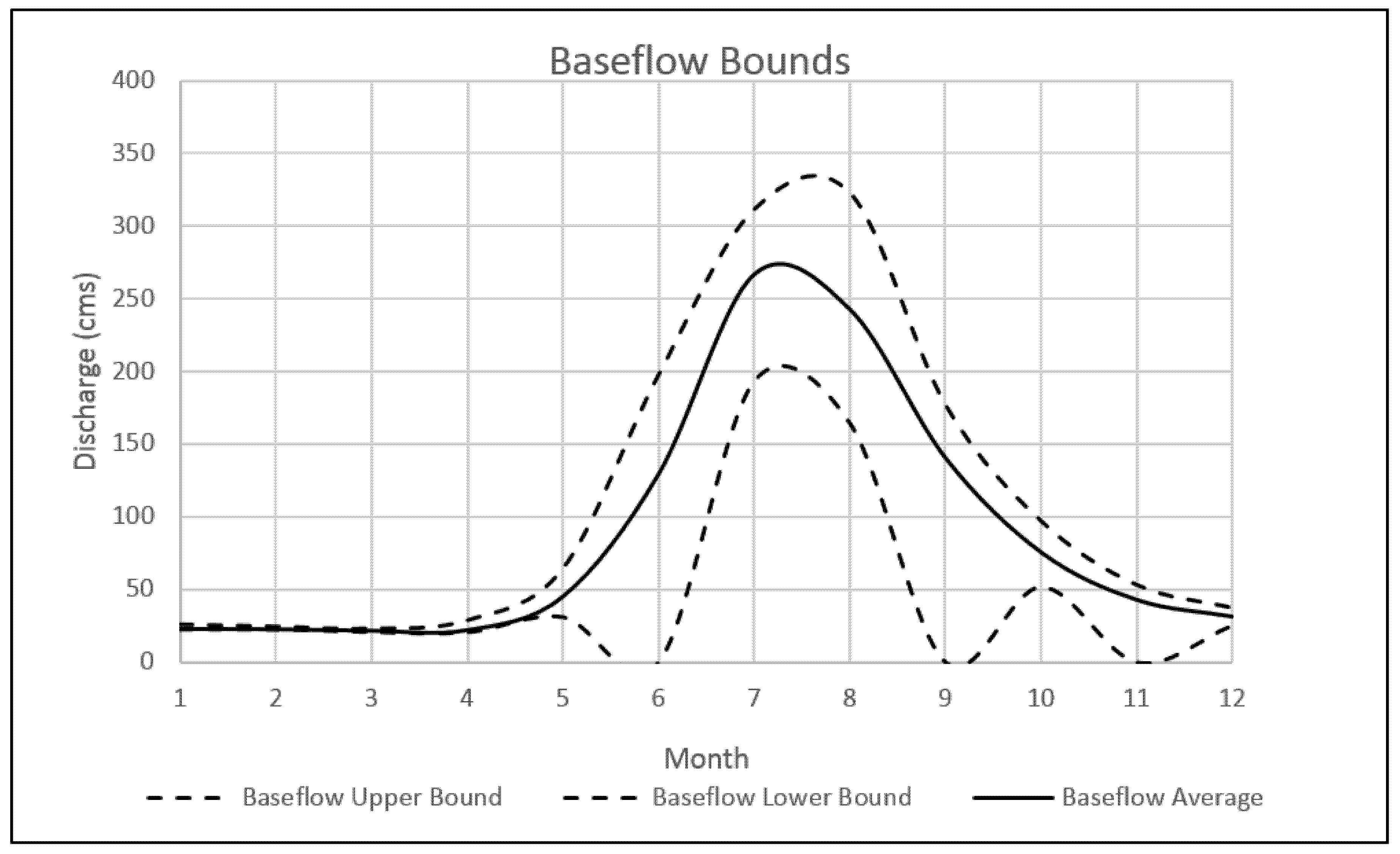
Direct baseflow information for the sub-basins that compose the Kenai River watershed is not available. To obtain the baseflow input for the HEC-HMS, available discharge information was analyzed to determine the minimum, average, and maximum of the minimum monthly flows. Assuming that the minimum flow is representative of the baseflow, the average baseflow was determined, along with the bounds of the baseflow. The results were then plotted to visualize the bounds of the baseflow. An example of these bounds is shown in Figure 2.
2.5. Impervious Surface
The impervious surface quantification for the Kenai River watershed and sub-basins was determined using the ESRI ArcGIS (GIS) software. Two datasets were used in GIS for quantification: the National Hydrography Database (NDH) water surface data, and the National Land Cover Database (NLCD) 2011 impervious development dataset. The impervious surface, due to development and waterbody impervious areas, was combined to create the sub-basin impervious area, which was then compared with the sub-basin area to determine the percentage of the sub-basin area that is impervious.
2.6. Surface Storage
Data on surface storage for grasses, shrubbery, and ground covering in the Kenai River watershed are not available in published works. All values used in the modeling efforts were estimated and calibrated. Starting values used in the estimation iterations were based on information found on water retention by grass [8].
2.7. Canopy Storage
Data on canopy storage in the Kenai River watershed are not directly available. To determine the canopy storage, initial values were chosen based on foliage types in the sub-basins. These foliage types were then referenced to the British Columbia forest hydrology guide, which has published precipitation interception values for various forest types [9].
2.8. Stream Function
The stream transform for each sub-basin is a calibrated time lag parameter in the HEC-HMS model. The calibration for this parameter was performed by comparing the model’s discharge peak time with the observed discharge peak time. The lagging of the peak was then applied to the model, so that the modeled peak discharge time coincided with the observed discharge peak time.
2.9. Soil Infiltration
Soil infiltration and loss estimates were calculated with the Soil Conservation Service (SCS) method and the impervious surface as found, as described above. The soil type was determined by referring to the United States Department of Agriculture (USDA) published soil survey [10]. Most soil data for the Kenai River watershed is available through published studies starting in 1918, with subsequent updates.
2.10. Lake Storage
Lake storage and elevation information are available through the Alaska Department of Fish and Game (ADF&G). Lakes used for fish spawning, or those that are stocked by ADF&G, have been surveyed, and bathymetric maps have been created [11]. To determine the volume of storage at a given lake depth, the bathymetric maps were georeferenced and overlaid on a mapping software. Elevation storage relationships were determined by tracing the depth contour lines, and multiplying them by the depth increments [12].
2.11. Evapotranspiration
Evapotranspiration (ET) for the Kenai River watershed was not analyzed in this modeling effort due to the lack of direct measurements of ET, prevailing low air temperatures, and the model being calibrated to single storm events, with reduced modeled time [13]. Thus, the ET was assumed to be negligible.
3. Modeling
3.1. Beaver Creek Sub-Basin
The Beaver Creek sub-basin, located near Kenai, Alaska, consists of several small low-gradient drainages. The sub-basin was separated into four separate drainages that feed into the main channel. These drainages are Timberlost Lake, Ootka Lake, Beaver Lake, and the Beaver Creek stream basin area. The HEC-HMS model was organized based on the layout determined from the topographic map delineation. Figure 3B shows the layout used in the HEC-HMS model for the Beaver Creek sub-basin. The input precipitation data for all sub-drainages within the Beaver Creek sub-basin were acquired from the Kenai Municipal Airport (Table 1). The modeled storms were approximately one week in duration and occurred in the early 1970’s, as seen the Figure 4, Figure 5 and Figure 6. This time period was chosen based on coinciding precipitation and discharge data at the site location. This setup was used in the creation of three sets of parameters that distinguish the difference in the basin hydrology during the spring, summer, and fall hydrologic regimes. Final model parameters used during spring, summer, and fall are available in the Supplementary Materials.
3.2. Russian River Sub-Basin
The Russian River sub-basin is split into two sub-drainages: the Upper Russian, that accounts for all the land upstream of the outlet of Lower Russian Lake, and the Lower Russian sub-drainage, that accounts for the area downstream of the Lower Russian Lake. With a single discharge gauge in the basin located at the outlet of Lower Russian Lake, the storage capacity of both the Upper and Lower Russian Lakes is combined to create a composite lake. The Upper Russian sub-drainage is routed through the stream length between the Upper and Lower Russian Lakes. The Upper Russian sub-drainage has a total area of 499.76 km2. The Lower Russian sub-drainage has an area of 166.59 km2. The Upper Russian Lake precipitation gauge data were used for modeling both the Upper Russian and Lower Russian sub-drainages. The configuration of the Russian River sub-basin in HEC-HMS is shown in Figure 3C. Final model parameters used for this sub-basin during spring, summer, and fall are available in Supplementary Materials.
3.3. Russian Lakes
The Russian Lakes reservoir uses the outflow curve [14] and the elevation-storage-discharge methods. These methods relate the elevation of the lake depth to its corresponding lake storage. The lake storage is then correlated to discharge. The primary relationship setting is storage-discharge, and the initial conditions are set so that inflow is equal to outflow. Due to the absence of a discharge gauge at the outlet of Upper Russian Lake, both Upper Russian Lake and Lower Russian Lake were combined to create a composite lake. The composite lake combined the depth and volume of both lakes in the sub-basin.
3.4. Ptarmigan Creek Sub-Basin
The Ptarmigan Creek sub-basin was split into two sub-drainages for modeling. Ptarmigan Creek Upper accounts for the area of Ptarmigan Lake and upstream, and Ptarmigan Creek Lower accounts for the area downstream of the lake. The area of Ptarmigan Creek Upper is 262.13 km2. Ptarmigan Creek Lower has an area of 87.39 km2. The model was arranged based on this information. Ptarmigan Creek sub-basin used the precipitation data from the Ptarmigan Lake precipitation gauge; the Grandview precipitation gauge was used for dates on which the Ptarmigan Lake gauge was inoperable. The configuration used in the HEC-HMS model for Ptarmigan Creek is shown in Figure 3A. Final model parameters used during spring, summer, and fall are available in Supplementary Materials.
3.5. Ptarmigan Lake
For Ptarmigan Lake, the model used the elevation-storage-discharge storage method. This method uses the outflow curve and the primary storage-discharge; the initial conditions were set so that inflow is equal to outflow conditions.
4. Results
4.1. Spring Beaver Creek
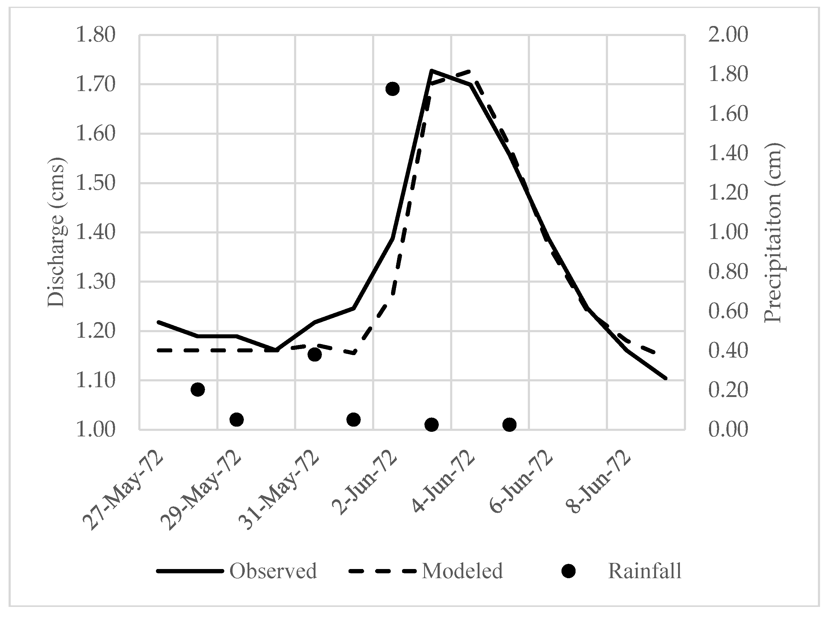
After calibration, the spring Beaver Creek modeled flows were very close to observed values. The period used to perform the calibration was 27 May 1972 through 9 June 1972. A discussion on the validity of calibrating this model to historic data from the 1970s is included later in the paper. During the calibration event, almost 2.5 cm (1 in) of rain fell across the basin. The maximum standard error of the daily modeled discharge over this period of study is approximately 8%. The averaged discharge standard error for the calibration of the model is 2.8%, and the standard error in the volume of throughput during the period is 1.6%, with a root mean square error of the discharge (RMSE-Q) of 0.048 cm. The observed versus modeled hydrograph can be seen in Figure 4.
4.2. Summer Beaver Creek
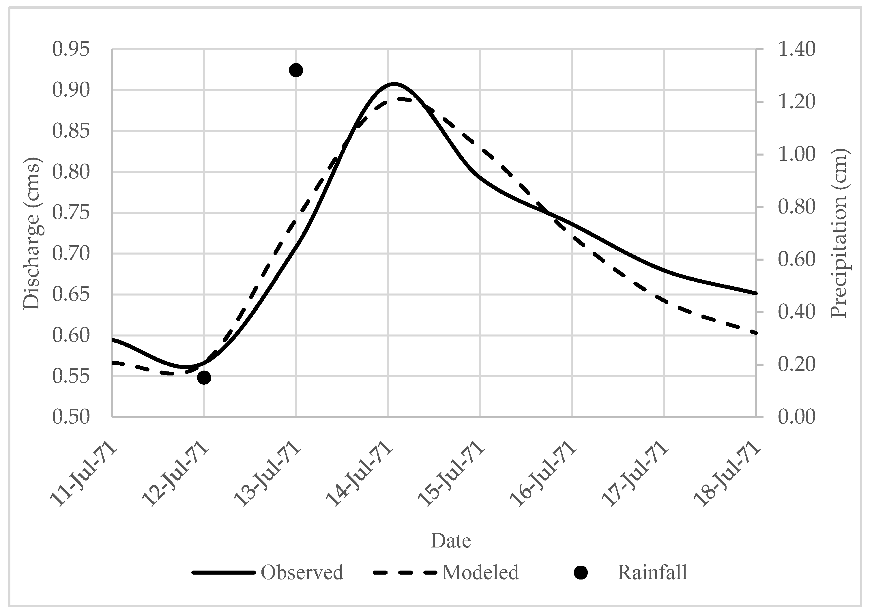
The summer modeling of Beaver Creek proved to be successful. The summer modeling calibration window used was 11 July 1971 through 18 July 1971. The summer calibration trial supports the spring calibration, since the hydrologic parameters remained constant except for those accounting for summer growth of vegetation. On the second and third days of this period, more than a 1.2 cm (0.5 in) of precipitation was measured at the nearest precipitation gauge to the sub-basin. With this precipitation applied to all sub-drainages within the sub-basin, the modeled outflow and observed discharge trended in the same pattern. The largest standard error on the daily discharge values for the modeling period is 7.4%. The averaged discharge standard errors are 3.9%, and the standard error in the volume is 1.4%, with an RMSE-Q of 0.031 cm. The observed versus modeled hydrograph can be seen in Figure 5.
4.3. Fall Beaver Creek
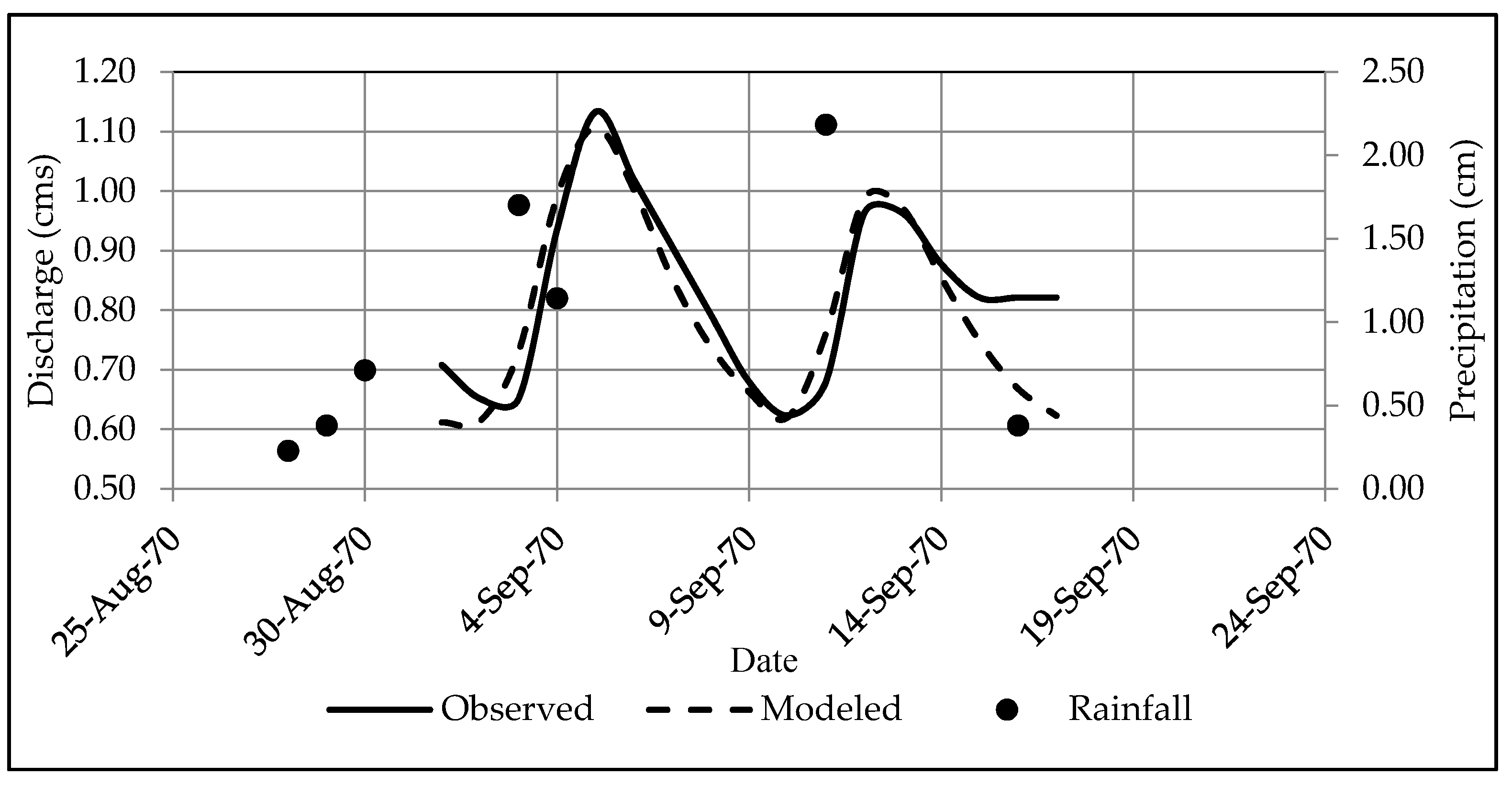
The fall calibration effort was the least successful of the Beaver Creek modeling work. The adjustments made to the parameters between seasonal modeling were limited mainly to adjustments to the surface and canopy storage. The fall modeling event supports the summer calibration trial. The modeling period used for the fall study extends from 28 August 1970 through 21 September 1970. The length of the modeling period is extended due to the length of a storm in the area. Storms of similar length to the spring and summer calibration periods were not available for times of coinciding precipitation and discharge measurements. The maximum daily standard error for the fall modeling period is 24%, the average daily standard error is 9.4%, and the standard error in volume is 6.6%, with an RMSE-Q of 0.091 cm. The precipitation over this time occurred in two peaks; total precipitation was 6.8 cm (2.69 in). The observed versus modeled hydrograph can be seen in Figure 6.
4.4. Russian River Sub-Basin
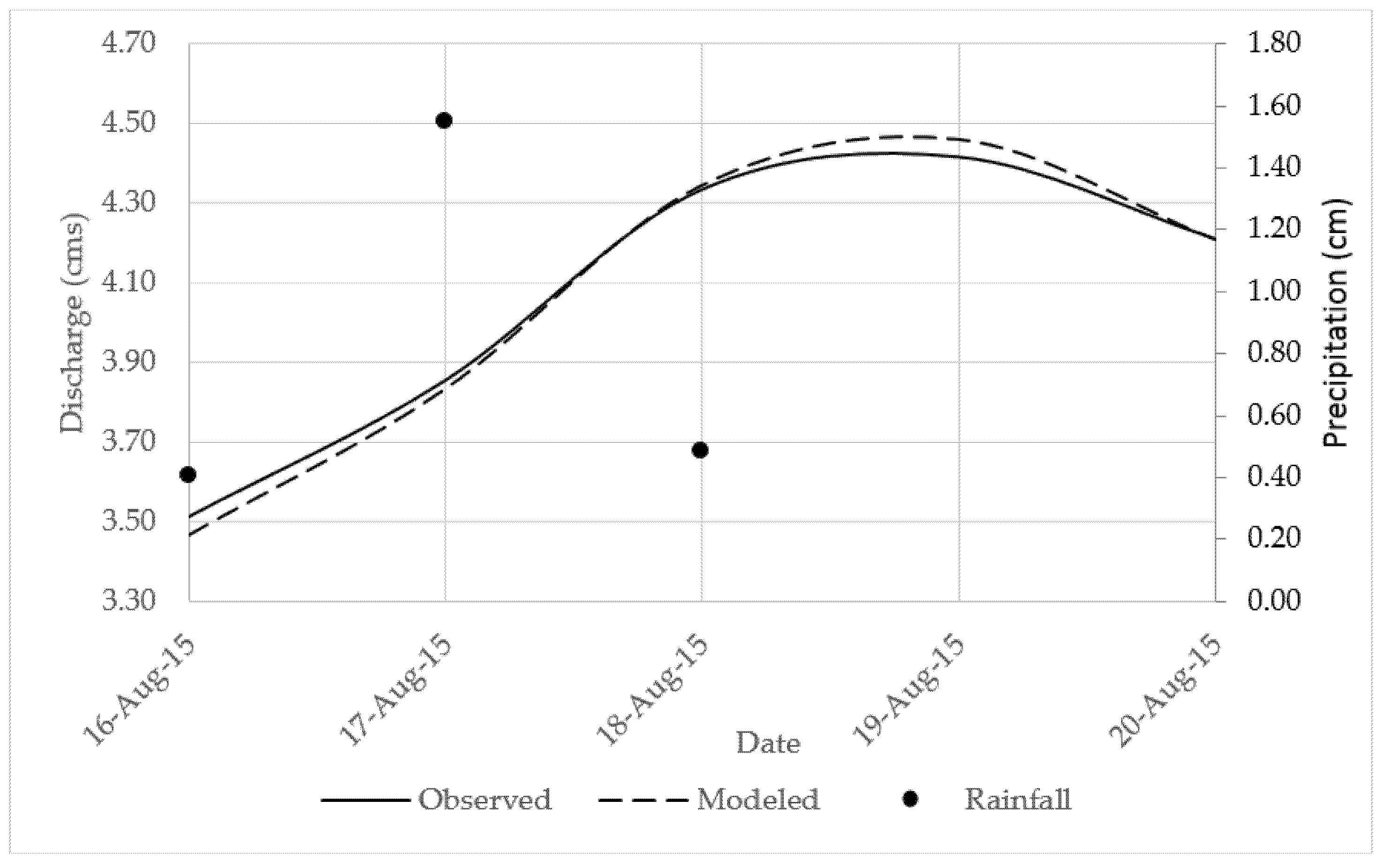
The Russian River calibration proved very successful for the modeling period. The period used was 15 August 2015 through 20 August 2015. During this time, over 2.54 cm (1 in) of precipitation fell on the sub-basin. The maximum daily standard error in the modeled discharge is 0.7%, and the average daily standard error is 0.3%, with a standard error in the volume of 0.2% over the modeling period, with an RMSE-Q of 0.013 cm. The observed versus modeled hydrograph can be seen in Figure 7.
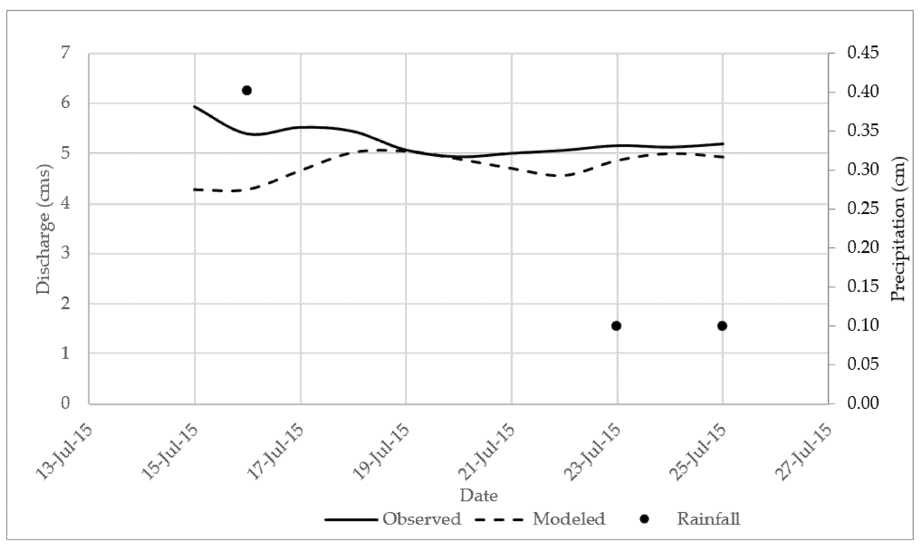
To validate the Russian River calibration, the model was applied to a second storm. The period modeled for the validation is 15 July 2015 to 25 July 2015. All parameters remained constant, and the average standard error in the discharge increased to 10%; the error in the volume increased to 10.1% with an RMSE-Q of 0.459 cm. The observed versus modeled hydrograph can be seen in Figure 8.
4.5. Ptarmigan Creek Sub-Basin
The Ptarmigan Creek calibration trends close to the observed data, with minor fluctuations in flow. The period modeled in the calibration is 16 August 2015 through 20 August 2015. During this time, almost 2.54 cm (1 in) of rainfall occurred. The maximum modeled daily discharge standard error is 1.3%, and the average daily discharge standard error is 0.6%. The standard error in the volume is 0.1% with an RMSE-Q of 0.031 cm. The observed versus modeled hydrograph can be seen in Figure 9.
The validation of the Ptarmigan Creek calibration occurred from 15 July 2015 to 25 July 2015. Since the period was outside the available data window for the Ptarmigan Lake precipitation gauge, data from the Grandview precipitation gauge were used for input. There were increases in both the average discharge error and the volume error. The average discharge standard error increased to 7.5%, and the volume standard error increased to 7.4% with an RMSE-Q of 0.71 cm. The observed versus modeled hydrograph can be seen in Figure 10.
5. Discussion
The Beaver Creek sub-basin modeled scenarios perform well under standard open-water seasons of late spring and summer, with errors of less than 4%. The model output follows the fluctuations in discharge over multiple peaks and low water levels. It was found that during the shoulder seasons of early spring and late fall, the model does not perform well, as the average error and volume error increased to 9.4% and 6.6%, respectively. The spring errors may be attributed to not accounting for snowmelt in the basin. Though the modeling windows were selected when the channels were ice-free, high-altitude snowmelt may have contributed to the overall observed discharge. The fall errors may be caused by errors in the estimation of storage in the wetlands, which comprise much of the sub-basin, or spatially differing precipitation to what was observed at the Kenai Municipal Airport. The adjustments made between the spring, summer, and fall modeling parameters account for the differing water storage and interception of the canopy and ground surface during these seasons, as well as differing system response time to precipitation events. The greatest variations are seen in the transition from spring to summer. The large changes to the parameters are speculated to be attributed to drying of the soils after spring snowmelt, and the growth of vegetation in and around the stream and basin.
With calibration of the model using data from the 1970s, a question could arise as to the validity of the use of the calibration for current and future modeling scenarios. As Bauret and Stuefer found, the precipitation trend has decreased since the mid-1960s [15]. Changes in the impervious surface due to increased land development were found to be 0.51% by interpolating the visual quantification of development from aerial photography [16]. The impervious surface in 1950 due to human development in the Kenai River watershed was 0.05%. This figure increased to 1.04% by the 1980s. The impervious surface in 2013 due to human development was found to be 1.28%, assuming a linear development of infrastructure between the 1950s and 1980s, and interpolated human development impervious of 0.71% for the 1970s. Thus, one could argue that the errors associated with increasing runoff due to increased development and the observed reductions in precipitation tend to balance out.
The Russian River sub-basin model performs well under the open-water season. The period of late spring to early fall produced acceptable results under the conditions present in the calibration year of 2015. Since flow data for lake discharge are limited, extreme precipitation events, whether high or low, have the potential to introduce errors in outflow calculations from the combined Russian Lakes.
Ptarmigan Creek sub-basin has reliable modeled output under average precipitation events. The narrow, steep-gradient basin has a large lake. Due to the positioning of the lake, and the runoff below the lake, the hydrograph increases steeply and then gradually decreases as the runoff drains from the lake. During the open-water season, the model reproduces peak flow due to lake outflow, and the modeled rate of decrease in the discharge follows the observed discharge closely. To achieve the steep rise in the hydrograph, the model required that the lower basin have a high level of flashiness. Thus, under heavy rainfall events, artificial peaks appear in the rise of the modeled hydrograph. This can be seen in the validation run of Ptarmigan Creek, where average errors increase to 7.6%, and volume errors increase to 7.4%, from the less than the 0.6% errors seen in the calibration event.
6. Conclusions
Sub-basin models have a variety of applications. With the use of modeled precipitation or predicted precipitation, stream flows could be estimated for use in fisheries studies. These studies could have an impact on economic planning for communities in the Kenai River watershed. As another application, the model could be used for exploring the effects of changing urbanization in the watershed area. As towns in the watershed increase in size, the percentage of impervious surface will increase with development, which will cause increased runoff during precipitation events, resulting in increased stream flow. With the landscape changes seen on the Kenai Peninsula, such as the wetland drying discussed by Berg et al., the effects of landscape changes on stream flow can be examined [17].
The sub-basin modeling effort successfully fulfilled the scope of the research task. However, to obtain a watershed-scale model that produces reasonable results, more information about the watershed must be collected. To address the gaps in information, a study of glacial melt and baseflow contributions to the hydrologic system is needed.
Supplementary Materials
The following are available online at https://www.mdpi.com/2073-4441/10/6/691/s1, Table S1: Beaver Creek Spring Parameters [3], Table S2: Beaver Creek Summer Parameters [3], Table S3: Beaver Creek Fall Parameters [3], Table S4: Russian River Parameters [3], Table S5: Ptarmigan Creek Parameters [3], Figure S1: Upper Russian Lake bathymetry [11], Figure S2: Lower Russian Lake bathymetry [11], Figure S3: Ptarmigan Lake bathymetry [11], Figure S4: Ptarmigan Lake storage-discharge relationship [3], Figure S5: Beaver Creek spring observed and modeled hydrographs [3], Figure S6: Beaver Creek summer observed and modeled hydrographs [3], Figure S7: Beaver Creek fall observed and modeled hydrographs [3], Figure S8: Russian River calibration observed and modeled hydrographs [3], Figure S9: Russian River validation observed and modeled hydrographs [3], Figure S10: Ptarmigan Creek calibration observed and modeled hydrographs [3], Figure S11: Ptarmigan Creek calibration observed and modeled hydrographs [3].
Author Contributions
Conceptualization, T.H.; Methodology, W.B.; Validation, W.B.; Formal Analysis, W.B.; Investigation, W.B; Resources, T.H.; Data Curation, W.B.; Writing-Original Draft Preparation, W.B.; Writing-Review & Editing, T.H.; Supervision, T.H.; Project Administration, T.H.; Funding Acquisition, T.H.
Funding
This research was partially funded by the National Science Foundation grant number 1208927 to the University of Alaska.
Conflicts of Interest
The authors declare no conflict of interest.
References
- Czarnezki, J.; Yaeger, J. On the River: A Guide to Owning and Managing Waterfront Property on the Kenai Peninsula; Kenai River Center: Soldotna, AK, USA, 2014. [Google Scholar]
- Kenai River Sportfishing Association. Fisheries Management: The Story of Salmon; Kenai River Sportfishing Association: Soldotna, AK, USA, 2016; Available online: https://www.krsa.com/fisheries-management.htm (accessed on 20 May 2015).
- Wells, B. Event Based Modeling Studying Three Sub-Basins in the Kenai River Watershed; University of Alaska Fairbanks: Fairbanks, AK, USA; ProQuest: Ann Arbor, MI, USA, 2016. [Google Scholar]
- Kenai Peninsula Economic Development District, Inc. 2016 Kenai Peninsula Situations and Prospects; Kenai Peninsula Economic Development District, Inc.: Nikiski, AK, USA, 2016. [Google Scholar]
- Kenai Peninsula Borough. Kenai Peninsula Borough Notes of Interest. 2016. Available online: http://www2.borough.kenai.ak.us/Econ/1S_P%20data/NotesofInterest/Climate.htm (accessed on 21 May 2015).
- Klein, E.; Berg, E.E.; Dial, R. Wetland Drying and Succession Across the Kenai Peninsula Lowland, South-Central Alaska. Can. J. For. Res. 2005, 35, 1931–1941. [Google Scholar] [CrossRef]
- Onset Computer Corporation. HOBO Rain Gauge Data Logger. Retrieved from Onset Monitoring Solutions. 2016. Available online: http://www.onsetcomp.com/products/data-loggers/rg3 (accessed on 10 June 2016).
- Abdul Wahab, N.; Mohd Tajuddin, R.; Tahir, W. Surface Water Retention Capacities of Different Grass Species for Storm Water Management. Int. Sustain. Civ. Eng. J. 2012, 1, 66–74. [Google Scholar]
- Pike, R.G.; Redding, T.E.; Moore, R.; Winkler, R.D.; Bladon, K.D. Compendium of Forest Hydrology and Geomorphology in British Columbia; Ministry of Forests and Range, Research Branch: Victoria, BC, Canadian, 2010.
- USDA. Urban Hydrology for Small Watersheds; Natural Resources Conservation Service, Conservation Engineering Division: Washington, DC, USA, 1986.
- Spafard, M.A.; Edmundson, J.A. A Morphometric Atlas of Alaskan Lakes: Cook Inlet, Prince William Sound, and Bristol Bay Areas; Alaska Department of Fish and Game, Commercial Fisheries: Anchorage, AK, USA, 2000. [Google Scholar]
- Wetzel, R.G. Limnology Lake and River Ecosystems; Academic Press: San Diego, CA, USA, 2001. [Google Scholar]
- Bedient, P.B.; Huber, W.C.; Vieux, B.E. Hydrology and Floodplain Analysis; Pearson Education, Inc.: Hoboken, NJ, USA, 2013. [Google Scholar]
- Wurbs, R.A.; James, W.P. Water Resources Engineering; Prentice Hall: Upper Saddle River, NJ, USA, 2002. [Google Scholar]
- Bauret, S.; Stuefer, S.L. Kenai Peninsula precipitation and air temperature trend analysis. In Proceedings of the 19th International Northern Research Basins Symposium and Workshop, University of Alaska Fairbanks, Fairbanks, AK, USA, 11–17 August 2013; pp. 35–45. [Google Scholar]
- Trammell, J. Assistant Professor of Environmental Studies. Wells, B. Interviewer. 10 November 2016. [Google Scholar]
- Berg, E.E.; Hillman, K.M.; Dial, R.; DeRuwe, A. Recent woody invasion of wetlands on the Kenai Peninsula Lowlands, South-Central Alaska: A major regime shift after 18,000 years of wet Sphagnum-sedge peat recruitment. Can. J. For. Res. 2009, 39, 2033–2046. [Google Scholar] [CrossRef]
Figure 1.
Kenai River Watershed with outlined sub-basins and selected sub-basins highlighted.

Figure 2.
Baseflow of the Kenai River as observed at Soldotna, Alaska discharge measurement station.
Figure 2.
Baseflow of the Kenai River as observed at Soldotna, Alaska discharge measurement station.

Figure 3.
Sub-basin model set-up.

Figure 4.
Observed and calibrated flows in Beaver Creek for the period 27 May 1972 through 9 June 1972.
Figure 4.
Observed and calibrated flows in Beaver Creek for the period 27 May 1972 through 9 June 1972.

Figure 5.
Observed and calibrated flows in Beaver Creek for the period 11 July 1971 through 18 July 1971.
Figure 5.
Observed and calibrated flows in Beaver Creek for the period 11 July 1971 through 18 July 1971.

Figure 6.
Observed and calibrated flows in Beaver Creek for the period 30 August 1970 through 17 September 1970.
Figure 6.
Observed and calibrated flows in Beaver Creek for the period 30 August 1970 through 17 September 1970.

Figure 7.
Observed and calibrated flows in Russian River for the period 15 August 2015 through 20 August 2015.
Figure 7.
Observed and calibrated flows in Russian River for the period 15 August 2015 through 20 August 2015.

Figure 8.
Observed and calibrated flows in Russian River for the period 15 July 2015 through 25 July 2015.
Figure 8.
Observed and calibrated flows in Russian River for the period 15 July 2015 through 25 July 2015.

Figure 9.
Observed and calibrated flows in Ptarmigan Creek for the period 16 August 2015 through 20 August 2015.
Figure 9.
Observed and calibrated flows in Ptarmigan Creek for the period 16 August 2015 through 20 August 2015.

Figure 10.
Observed and calibrated flows in Ptarmigan Creek for the period 15 July 2015 through 25 July 2015.
Figure 10.
Observed and calibrated flows in Ptarmigan Creek for the period 15 July 2015 through 25 July 2015.


Table 1.
Precipitation Gauges.
| Gauge Name | Station ID | Latitude | Longitude | Coverage (%) | Period of Record |
|---|---|---|---|---|---|
| Kenai Municipal Airport | USW00026523 | 60.58 | −151.24 | 70% | 01/05/1899–Present |
| Ptarmigan Creek | N/A | 60.41 | −149.3 | N/A | 10/08/2015–18/09/2015 |
| Russian River | N/A | 60.36 | −149.89 | N/A | 15/05/2015–19/09/2015 |
Table 2.
Streamflow Gauge Site Information.
| Stream Name | Gauge ID Number | Latitude | Longitude | Period of Record |
|---|---|---|---|---|
| Ptarmigan Creek (Historic) | USGS1524400 | 60.41 | −149.36 | 01/05/1947–13/09/1958 |
| Russian River (Historic) | USGS15264000 | 60.45 | −149.98 | 01/05/1947–13/09/1958 |
| Beaver Creek (Historic) | USGS15266500 | 60.56 | −151.12 | 01/10/1967–13/09/1978 |
© 2018 by the authors. Licensee MDPI, Basel, Switzerland. This article is an open access article distributed under the terms and conditions of the Creative Commons Attribution (CC BY) license (http://creativecommons.org/licenses/by/4.0/).
Share and Cite
MDPI and ACS Style
Wells, B.; Toniolo, H. Hydrologic Modeling of Three Sub-Basins in the Kenai River Watershed, Alaska, USA. Water 2018, 10, 691. https://doi.org/10.3390/w10060691
AMA Style
Wells B, Toniolo H. Hydrologic Modeling of Three Sub-Basins in the Kenai River Watershed, Alaska, USA. Water. 2018; 10(6):691. https://doi.org/10.3390/w10060691
Chicago/Turabian StyleWells, Brett, and Horacio Toniolo. 2018. "Hydrologic Modeling of Three Sub-Basins in the Kenai River Watershed, Alaska, USA" Water 10, no. 6: 691. https://doi.org/10.3390/w10060691
Note that from the first issue of 2016, this journal uses article numbers instead of page numbers. See further details here.