Managing Salinity in Upper Colorado River Basin Streams: Selecting Catchments for Sediment Control Efforts Using Watershed Characteristics and Random Forests Models

 , , and
Abstract
:1. Introduction
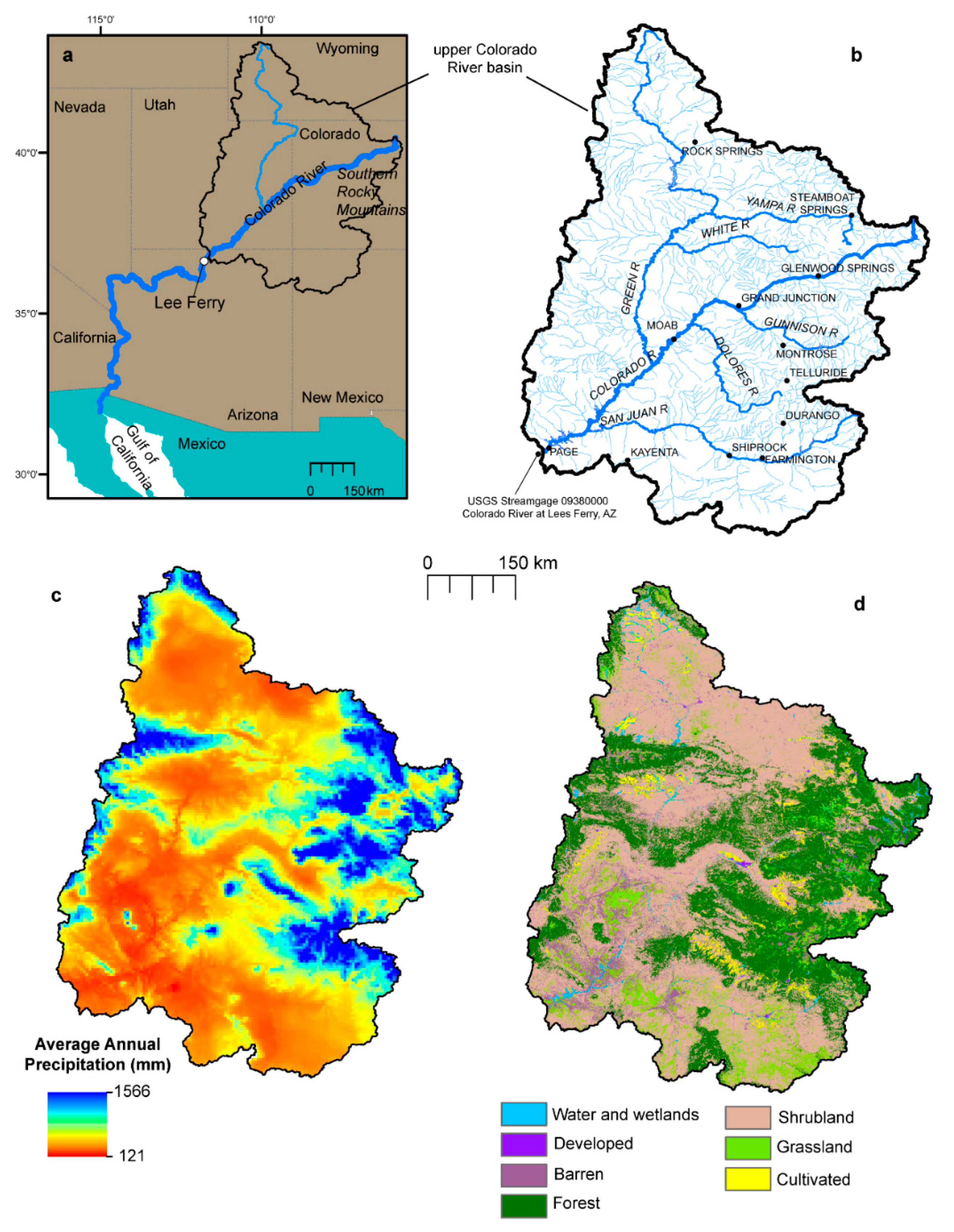
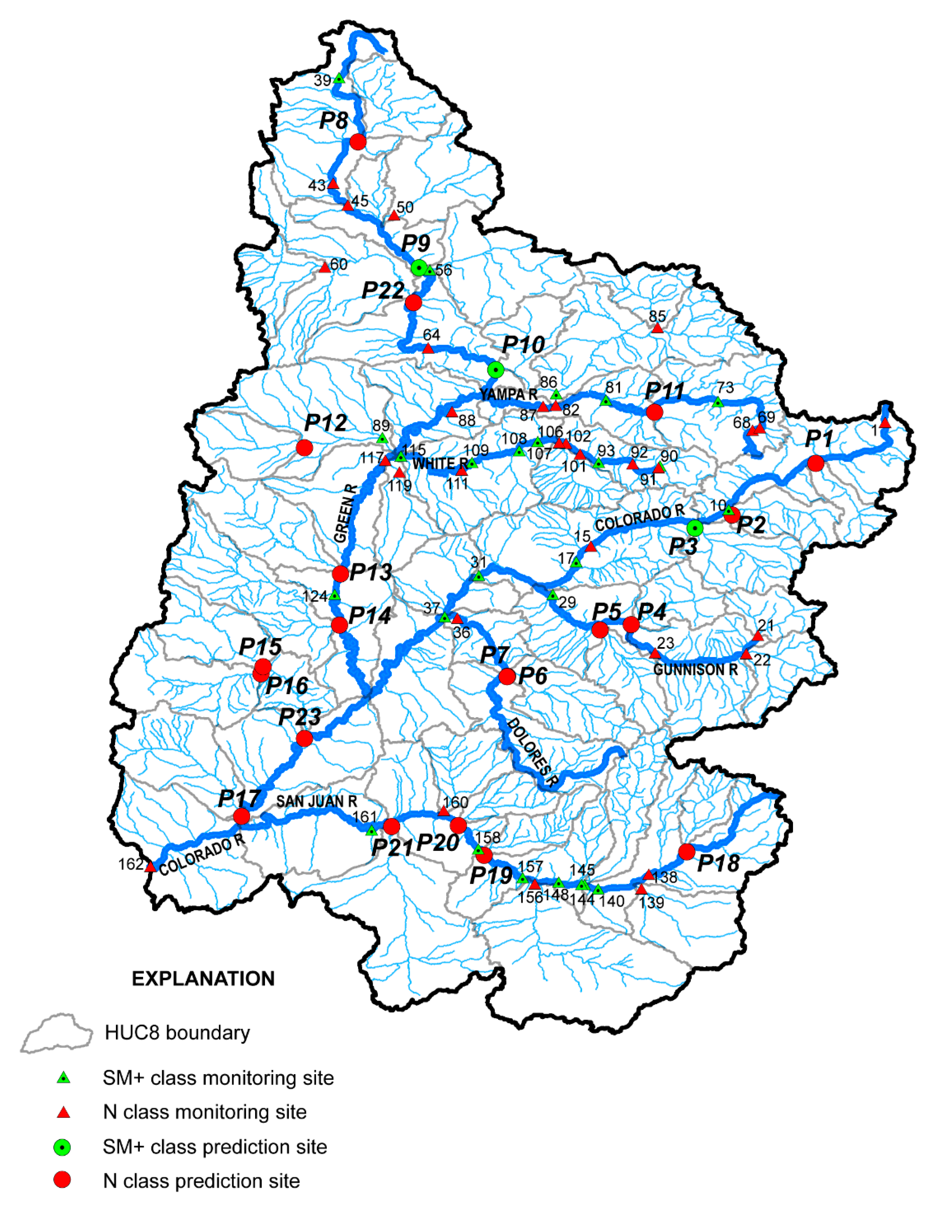
1.1. Study Area
1.2. Dissolved Solids and Suspended Sediment in the UCRB
2. Materials and Methods
2.1. Watershed Characteristics Data
2.2. Model Development
2.3. Use of Random Forests Class-Prediction Model
3. Results and Discussion
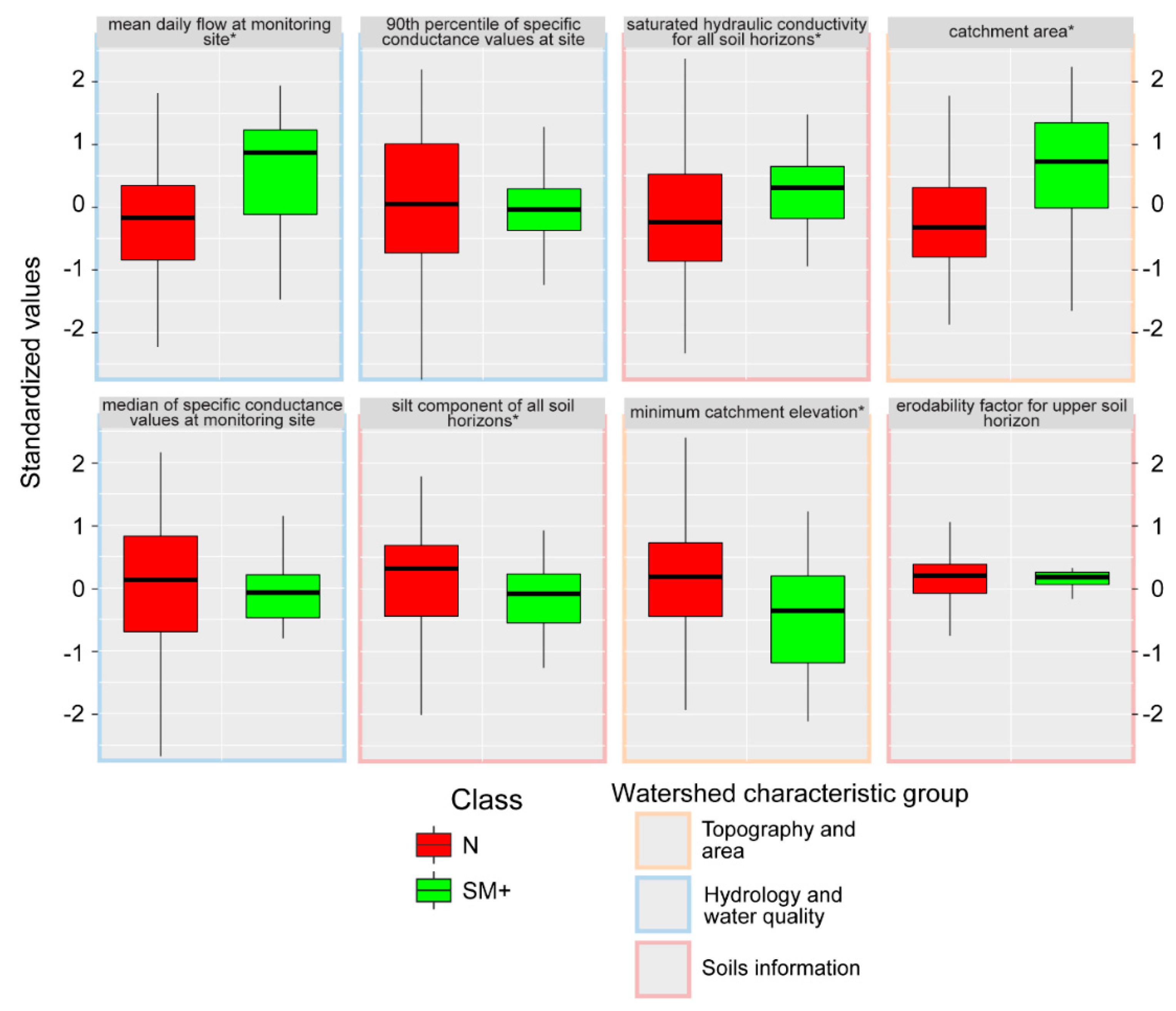
3.1. Exploratory Random Forests Model
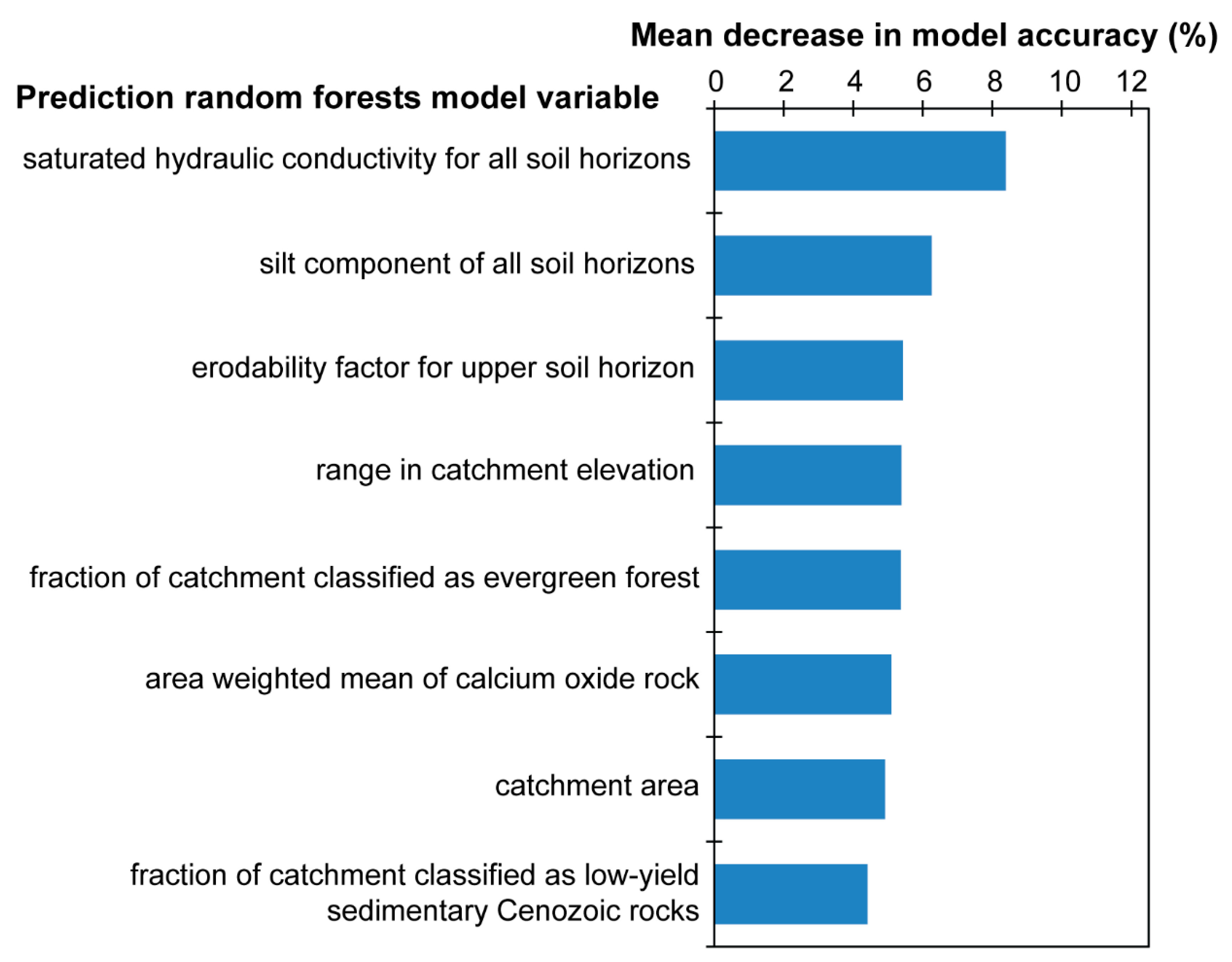
3.2. Predictive Random Forests Model
3.3. Model Application
4. Summary and Conclusions
Supplementary Materials
Author Contributions
Acknowledgments
Conflicts of Interest
References
- Bureau of Reclamation. Quality of Water, Colorado River Basin; Bureau of Reclamation Progress Report No. 23; Bureau of Reclamation: Washington, DC, USA, 2011; 76p. Available online: https://www.usbr.gov/uc/progact/salinity/pdfs/PR23final.pdf (accessed on 9 April 2018).
- Colorado River Basin Salinity Control Forum. Colorado River Basin Salinity Control Program Briefing Document; Colorado River Basin Salinity Control Forum: Bountiful, UT, USA, 2013; 4p, Available online: http://www.coloradoriversalinity.org/docs/CRBSCP%20Briefing%20Document%202013%20Feb%204.pdf (accessed on 9 April 2018).
- Colorado River Basin Salinity Control Forum. Water quality standards for salinity. In Colorado River System, 2011 Review; Colorado River Basin Salinity Control Forum: Bountiful, UT, USA, 2011; 99p, Available online: http://www.coloradoriversalinity.org/docs/2011%20REVIEW-October.pdf (accessed on 9 April 2018).
- Anning, D.W.; Bauch, N.J.; Gerner, S.J.; Flynn, M.E.; Hamlin, S.N.; Moore, S.J.; Schaefer, D.H.; Anderholm, S.K.; Spangler, L.E. Dissolved Solids in Basin-Fill Aquifers and Streams in the Southwestern United States; U.S. Geological Survey Scientific Investigations Report 2006-5315, 2007, Revised 2010; U.S. Geological Survey: Reston, VA, USA, 2007; 168p. Available online: http://pubs.usgs.gov/sir/2006/5315/ (accessed on 9 April 2018).
- Hawkins, R.H.; Gifford, G.F.; Jurinak, J.J. Effects of Land Processes on the Salinity of the Upper Colorado River Basin: Final Project Report; Bureau of Land Management Contract No. 52500-CT5-16; Bureau of Land Management: Washington, DC, USA, 1977; 206p. Available online: http://archive.org/details/effectsoflandpro00hawk (accessed on 9 April 2018).
- Schumm, S.A.; Gregory, D.I. Diffuse-Source Salinity: Mancos Shale Terrain; Bureau of Land Management Report No. BLM-YA-PT-86-008-4341; Bureau of Land Management Service Center: Lakewood, CO, USA, 1986; 196p. Available online: http://archive.org/details/diffusesourcesal00schu (accessed on 9 April 2018).
- Cloern, J.E.; Powell, T.M.; Huzzey, L.M. Spatial and temporal variability in South San Francisco Bay (USA). II. Temporal changes in salinity, suspended sediments, and phytoplankton biomass and productivity over tidal time scales. Estuar. Coast. Shelf Sci. 1989, 28, 599–613. [Google Scholar] [CrossRef]
- Lane, R.R.; Day, J.W.; Marx, B.D.; Reyes, E.; Hyfield, E.; Day, J.N. The effects of riverine discharge on temperature, salinity, suspended sediment and chlorophyll a in a Mississippi delta estuary measured using a flow-through system. Estuar. Coast. Shelf Sci. 2007, 74, 145–154. [Google Scholar] [CrossRef]
- Powell, T.M.; Cloern, J.E.; Huzzey, L.M. Spatial and temporal variability in South San Francisco Bay (USA). I. Horizontal distributions of salinity, suspended sediments, and phytoplankton biomass and productivity. Estuar. Coast. Shelf Sci. 1980, 28, 583–597. [Google Scholar] [CrossRef]
- Prandle, D.; Hydes, D.J.; Jarvis, J.; McManus, J. The seasonal cycles of temperature, salinity, nutrients and suspended sediment in the southern North Sea in 1988 and 1989. Estuar. Coast. Shelf Sci. 1997, 45, 669–680. [Google Scholar] [CrossRef]
- Uncles, R.T.; Elliott, R.C.A.; Weston, S.A. Dispersion of salt and suspended sediment in a partly mixed estuary. Estuaries 1985, 8, 256–269. [Google Scholar] [CrossRef]
- Uncles, R.T.; Elliott, R.C.A.; Weston, S.A. Observed fluxes of water, salt and suspended sediment in a partly mixed estuary. Estuar. Coast. Shelf Sci. 1985, 20, 147–167. [Google Scholar] [CrossRef]
- Gibbs, R.J. The geochemistry of the Amazon River system: Part I. The factors that control the salinity and the composition and concentration of the suspended solids. Geol. Soc. Am. Bull. 1967, 78, 1203–1232. [Google Scholar] [CrossRef]
- Guyot, J.L.; Filizola, N.; Quintanilla, J.; Cortez, J. Dissolved Solids and Suspended Sediment Yields in the Rio Madeira Basin, from the Bolivian Andes to the Amazon; Erosion and Sediment Yield: Global and Regional Perspectives, IAHS Publication No. 236; IAHS: London, UK, 1996; pp. 55–63. Available online: http://hydrologie.org/redbooks/a236/iahs_236_0055.pdf (accessed on 9 April 2018).
- Hubbard, R.K.; Sheridan, J.M.; Marti, L.R. Dissolved and suspended solids transport from coastal plain watersheds. J. Environ. Qual. 1990, 19, 413–420. [Google Scholar] [CrossRef]
- Lewis, W.M.; Saunders, J.F. Concentration and transport of dissolved and suspended substances in the Orinoco River. Biogeochemistry 1989, 7, 203–240. [Google Scholar] [CrossRef]
- Moore, S.J.; Anderholm, S.K. Spatial and Temporal Variations in Streamflow, Dissolved Solids, Nutrients, and Suspended Sediment in the Rio Grande Valley Study Unit, Colorado, New Mexico, and Texas, 1993–1995; Geological Survey Water-Resources Investigations Report 02-4224; U.S. Geological Survey: Albuquerque, NM, USA, 2002; 58p. Available online: http://pubs.usgs.gov/wri/wri02-4224/pdf/wrir02-4224.pdf (accessed on 8 April 2018).
- Nagano, T.; Yanase, N.; Tsuduki, K.; Nagao, S. Particulate and dissolved elemental loads in the Kuji River related to discharge rate. Environ. Int. 2003, 28, 649–658. [Google Scholar] [CrossRef]
- Reynolds, B. A comparison of element outputs in solution, suspended sediments and bedload for a small upland catchment. Earth Surf. Proc. Land. 1986, 11, 217–221. [Google Scholar] [CrossRef]
- Roy, S.; Gaillardet, J.; Allegre, C.J. Geochemistry of dissolved and suspended loads of the Seine river, France: Anthropogenic impact, carbonate and silicate weathering. Geochim. Cosmochim. Acta 1999, 63, 1277–1292. [Google Scholar] [CrossRef]
- Subramanian, V. Chemical and suspended-sediment characteristics of rivers of India. J. Hydrol. 1979, 44, 37–55. [Google Scholar] [CrossRef]
- Tillman, F.D.; Anning, D.W. A data reconnaissance on the effect of suspended-sediment concentrations on dissolved-solids concentrations in rivers and tributaries in the Upper Colorado River Basin. J. Hydrol. 2014, 519, 1020–1030. [Google Scholar] [CrossRef]
- James, G.; Witten, D.; Hastie, T.; Tibshirani, R. An Introduction to Statistical Learning with Applications in R; Springer Science + Business Media: New York, NY, USA, 2013; ISBN 978-1-4614-7138-7. [Google Scholar]
- Breiman, L. Random forests. Mach. Learn. 2001, 45, 5–32. [Google Scholar] [CrossRef]
- Cutler, D.R.; Edwards, T.C.; Beard, K.H.; Cutler, A.; Hess, K.T.; Gibson, J.; Lawler, J.J. Random forests for classification in ecology. Ecology 2007, 88, 2783–2792. [Google Scholar] [CrossRef] [PubMed]
- Murphy, M.A.; Evans, J.S.; Storfer, A. Quantifying Bufo boreas connectivity in Yellowstone National Park with landscape genetics. Ecology 2010, 91, 252–261. [Google Scholar] [CrossRef] [PubMed]
- Prasad, A.M.; Iverson, L.R.; Liaw, A. Newer classification and regression tree techniques: Bagging and Random Forests for Ecological Prediction. Ecosystems 2006, 9, 181–199. [Google Scholar] [CrossRef]
- Kronholm, S.C.; Capel, P.D.; Terziotti, S. Statistically extracted fundamental watershed variables for estimating loads of total nitrogen in small streams. Environ. Model. Assess. 2016, 21, 681–690. [Google Scholar] [CrossRef]
- Reynolds, L.V.; Shafroth, P.B.; Poff, N.L. Modeled intermittency risk for small streams in a North American river basin under climate change. J. Hydrol. 2015, 523, 768–780. [Google Scholar] [CrossRef]
- Nolan, B.T.; Gronberg, J.M.; Faunt, C.C.; Eberts, S.M.; Belitz, K. Modeling nitrate at domestic and public-supply well depths in the Central Valley, California. Environ. Sci. Technol. 2014, 48, 5643–5651. [Google Scholar] [CrossRef] [PubMed]
- Olson, J.R.; Hawkins, C.P. Predicting natural base-flow stream water chemistry in the western United States. Water Resour. Res. 2012, 48, W02504. [Google Scholar] [CrossRef]
- Lee, Y.J.; Park, C.; Lee, M.L. Identification of a contaminant source location in a river system using random forests models. Water 2018, 10, 391. [Google Scholar] [CrossRef]
- Feng, Q.; Liu, J.; Gong, J. Urban flood mapping based on unmanned aerial vehicle remote sensing and random forest classifier—A Case of Yuyao, China. Water 2015, 7, 1437–1455. [Google Scholar] [CrossRef]
- Elith, J.; Leathwick, J.R.; Hastie, T. A working guide to boosted regression trees. J. Anim. Ecol. 2008, 77, 802–813. [Google Scholar] [CrossRef] [PubMed]
- Liaw, A.; Weiner, M. Classification and regression by random Forest. R News 2002, 2/3, 18–22. Available online: https://www.r-project.org/doc/Rnews/Rnews_2002-3.pdf (accessed on 9 April 2018).
- PRISM Climate Group. Oregon State University, Digital Climate Data. 2012. Available online: http://prism.oregonstate.edu/ (accessed on 15 January 2012).
- Fry, J.; Xian, G.; Jin, S.; Dewitz, J.; Homer, C.; Yang, L.; Barnes, C.; Herold, N.; Wickham, J. Completion of the 2006 national land cover database for the conterminous United States. Photogramm. Eng. Remote Sens. 2011, 77, 858–864. Available online: http://www.mrlc.gov/downloadfile2.php?file=September2011PERS.pdf (accessed on 9 April 2018).
- Anderson, D.L. History of the development of the Colorado River and ‘The law of the River’. Water Resour. Environ. Hist. 2004, 75–81. [Google Scholar] [CrossRef]
- Liebermann, T.D.; Mueller, D.K.; Kircher, J.E.; Choquette, A.F. Characteristics and Trends of Streamflow and Dissolved Solids in the Upper Colorado River Basin, Arizona, Colorado, New Mexico, Utah, and Wyoming; U.S. Geological Survey Water-Supply Paper 2358; U.S. Geological Survey: Denver, CO, USA, 1989; 64p. Available online: http://pubs.usgs.gov/wsp/2358/report.pdf (accessed on 9 April 2018).
- Kenney, T.A.; Gerner, S.J.; Buto, S.G.; Spangler, L.E. Spatially Referenced Statistical Assessment of Dissolved-Solids Load Sources and Transport in Streams of the Upper Colorado River Basin; U.S. Geological Survey Scientific Investigations Report 2009–5007; U.S. Geological Survey: Reston, VA, USA, 2009; 50p. Available online: http://pubs.usgs.gov/sir/2009/5007 (accessed on 9 April 2018).
- Tuttle, M.L.; Grauch, R.I. Salinization of the Upper Colorado River—Fingerprinting Geologic Salt Sources; U.S. Geological Survey Scientific Investigations Report 2009–5072; U.S. Geological Survey: Reston, VA, USA, 2009; 70p. Available online: https://pubs.usgs.gov/sir/2009/5072/ (accessed on 9 April 2018).
- Lieb, K.J.; Linard, J.I.; Williams, C.A. Statistical Relations of Salt and Selenium Loads to Geospatial Characteristics of Corresponding Subbasins of the Colorado and Gunnison rivers in Colorado; U.S. Geological Survey Scientific Investigations Report 2012–5003; U.S. Geological Survey: Reston, VA, USA, 2012; 31p. Available online: https://pubs.usgs.gov/sir/2012/5003/ (accessed on 9 April 2018).
- Laronne, J.B. Evaluation of the Storage of Diffuse Sources of Salinity in the Upper Colorado River Basin; Colorado Water Resources Research Institute Completion Report 79; Environmental resources center: Fort Collins, CO, USA, 1977; 122p, Available online: http://www.cwi.colostate.edu/publications/cr/79.pdf (accessed on 9 April 2018).
- Liaw, A.; Weiner, M. Breiman and Cutler’s Random Forests for Classification and Regression, Package Description. 2015. Available online: https://cran.r-project.org/web/packages/randomForest/randomForest.pdf (accessed on 9 April 2018).
- R Development Core Team. R: A Language and Environment for Statistical Computing; R Foundation for Statistical Computing: Vienna, Austria, 2013; Available online: http://www.r-project.org/ (accessed on 9 April 2018).
- U.S. Geological Survey. Boundary Descriptions and Names of Regions, Subregions, Accounting Units and Cataloging Units. 2016. Available online: https://water.usgs.gov/GIS/huc_name.html#Region14 (accessed on 9 April 2018).


| Model Argument | Argument Values |
|---|---|
| mtry | integers from 1 to 18 |
| nodesize | integers from 1 to 20 |
| classwt | integers from 1 to 50 for N class integers from 100 to 50 for SM+ class |
| cutoff | 0.99 to 0.5 for N class 0.01 to 0.5 for SM+ class |
| Classification from Tillman and Anning [22] | Random Forests Predicted Class | Class Error | |
|---|---|---|---|
| N | SM+ | ||
| N class | 96 | 23 | 19.3% |
| SM+ class | 10 | 34 | 22.7% |
| Classification from Tillman and Anning [22] | Random Forests Predicted Class | Class Error | |
|---|---|---|---|
| N | SM+ | ||
| N class | 107 | 12 | 10.1% |
| SM+ class | 18 | 26 | 40.9% |
© 2018 by the authors. Licensee MDPI, Basel, Switzerland. This article is an open access article distributed under the terms and conditions of the Creative Commons Attribution (CC BY) license (http://creativecommons.org/licenses/by/4.0/).
Share and Cite
Tillman, F.D.; Anning, D.W.; Heilman, J.A.; Buto, S.G.; Miller, M.P. Managing Salinity in Upper Colorado River Basin Streams: Selecting Catchments for Sediment Control Efforts Using Watershed Characteristics and Random Forests Models. Water 2018, 10, 676. https://doi.org/10.3390/w10060676
Tillman FD, Anning DW, Heilman JA, Buto SG, Miller MP. Managing Salinity in Upper Colorado River Basin Streams: Selecting Catchments for Sediment Control Efforts Using Watershed Characteristics and Random Forests Models. Water. 2018; 10(6):676. https://doi.org/10.3390/w10060676
Chicago/Turabian StyleTillman, Fred D., David W. Anning, Julian A. Heilman, Susan G. Buto, and Matthew P. Miller. 2018. "Managing Salinity in Upper Colorado River Basin Streams: Selecting Catchments for Sediment Control Efforts Using Watershed Characteristics and Random Forests Models" Water 10, no. 6: 676. https://doi.org/10.3390/w10060676