Numerical Study of Spatial Behavior of Solute Particle Transport in Single Fracture with Variable Apertures


1
Department of Architecture, Sejong University, 209, Neungdong-ro, Gwangjin-gu, Seoul 143-747, Korea
2
Department of Civil Engineering, Kyungnam University, 7, Kyungnamdaehak-ro, Masanhappo-gu, Changwon 631-701, Korea
*
Author to whom correspondence should be addressed.
Water 2018, 10(6), 673; https://doi.org/10.3390/w10060673
Submission received: 1 March 2018
/
Revised: 18 May 2018
/
Accepted: 22 May 2018
/
Published: 23 May 2018
(This article belongs to the Special Issue Water Resources Investigation: Geologic Controls on Groundwater Flow)
Abstract
:The aim of this study is to numerically analyze spatial behaviors of solute particle transport in a single fracture with spatially correlated variable apertures under application of effective normal stress conditions. The numerical results show that solute particle transport in a single fracture is strongly affected by spatial correlation length of variable apertures and applied effective normal stress. As spatial correlation length increases, mean residence time of solute particles decreases and tortuosity and Peclet number (a dimensionless number representing the relationship between the rate of advection of solute particles by the flow and the rate of diffusion of solute particles) also decreases. These results indicate that the geometry of the aperture distribution is favorable to solute particle transport when the spatial correlation length is increased. However, as effective normal stress increases, the mean residence time and tortuosity tend to increase but the Peclet number decreases. The main reason for a decreasing Peclet number is that the solute particle is transported by one or two channels with relatively higher localized flow rates owing to increase in contact areas resulting from increasing effective normal stress. Based on the numerical results of the solute particle transport produced in this study, an exponential-type correlation formula between the mean residence time and the effective normal stress is proposed.
1. Introduction
The analysis of the fluid flow and solute transport in a single fracture is significant as it provides useful information for assessing groundwater flow and movement of pollutants through crystalline bedrock and for predicting the possible route of radioactive substances that have leaked from radioactive waste disposal facilities into deep underground levels. A number of studies on fluid flow and solute transport in a single fracture has been conducted so far and include laboratory or field experiments [1,2,3,4,5,6,7,8] and numerical experiments [9,10,11,12,13].
It is known that fluid flow and solute transport in a rough single fracture is significantly affected by the spatial variation of the aperture distribution owing to roughness and contact surfaces of the fracture walls [12,14]. Such a spatially variable aperture results in a “channeling effect”, which means that fluid and solute move through a relatively large aperture [12,15]. In addition, the effect of the effective normal stress, which acts vertically against the fracture surfaces, increases the contact areas between the fracture walls, thereby reducing the aperture distribution available for fluid flow or solute transport. These two phenomena eventually increase the tortuosity of fluid flow and solute transport owing to reduced flow passing through a single fracture and connections between apertures.
Thompson [13] demonstrated that the velocity of solute transport tends to be higher or lower than the mean flow velocity depending on the roughness of the fracture walls and contact surfaces. Jeong and Song [10] conducted a numerical study on flows and solute transport in a rough fracture with an anisotropic aperture distribution, and Tsang et al. [14] numerically studied the spatial dispersion of a solute transported through a channel with one-dimensionally changing apertures. Ewing and Jaynes [16] also conducted extensive numerical studies on factors such as size of the fracture and shape of the mesh that affect solute transport in a single fracture, and Jeong and Song [10] examined fluid flow and solute transport in a single fracture with variable aperture distribution that is generated using fractal technique. Recently, Vogler et al. [17] presented the fully coupled hydro-mechanical method to investigate the effect of fracture heterogeneity on fluid flow through fractures at laboratory scale but they did not consider solute transport in fractures with hydro-mechanical effect.
In this study, spatial behaviors of solute particle transport in a single fracture with a variable aperture distribution, which depend on the spatial correlation and effective normal stress, were numerically investigated. The aim of this study is to propose a new empirical formula to describe the relationship between mean residence time of solute particles and effective normal stress. The mean residence time in the proposed empirical formula can be derived by analysis of breakthrough curves for each level of effective normal stress and spatial correlation ratio.
2. Solute Transport Model: Random Walk Particle Following (RWPF) Model
In this study, it is assumed that solute transport through spatially varying apertures occurs in a one-dimensional channel that connects individual elements constituting a single fracture. The numerical simulation of solute particle transport was conducted using the random walk particle following (RWPF) model [18]. This model was originally developed to simulate solute particle transport in three-dimensional discrete fracture networks with a large number of individual fractures (e.g., more than 10,000). The merit of this model—compared to the existing random walk particle tracking (RWPT) model LaBolle et al. [11]—is that it does not require discrete mathematics for time calculation, thereby increasing the efficiency of calculation when a large number of fractures is generated within a given space.
In the RWPF model, the spatial distribution of solute particles is determined through a stochastic process. The probability density function for residence time of solute particles in RWPF model is
where [m] refers to the length of the one-dimensional channel, [m2/sec] to the longitudinal dispersion coefficient, [m/sec] to the mean velocity, and [sec] to time.
The standard deviation of the spatial transport through the distribution of particles within a one-dimensional channel is expressed as a function of longitudinal dispersion coefficient and time:
The residence time of solute particles that are moved in the flow field is calculated as:
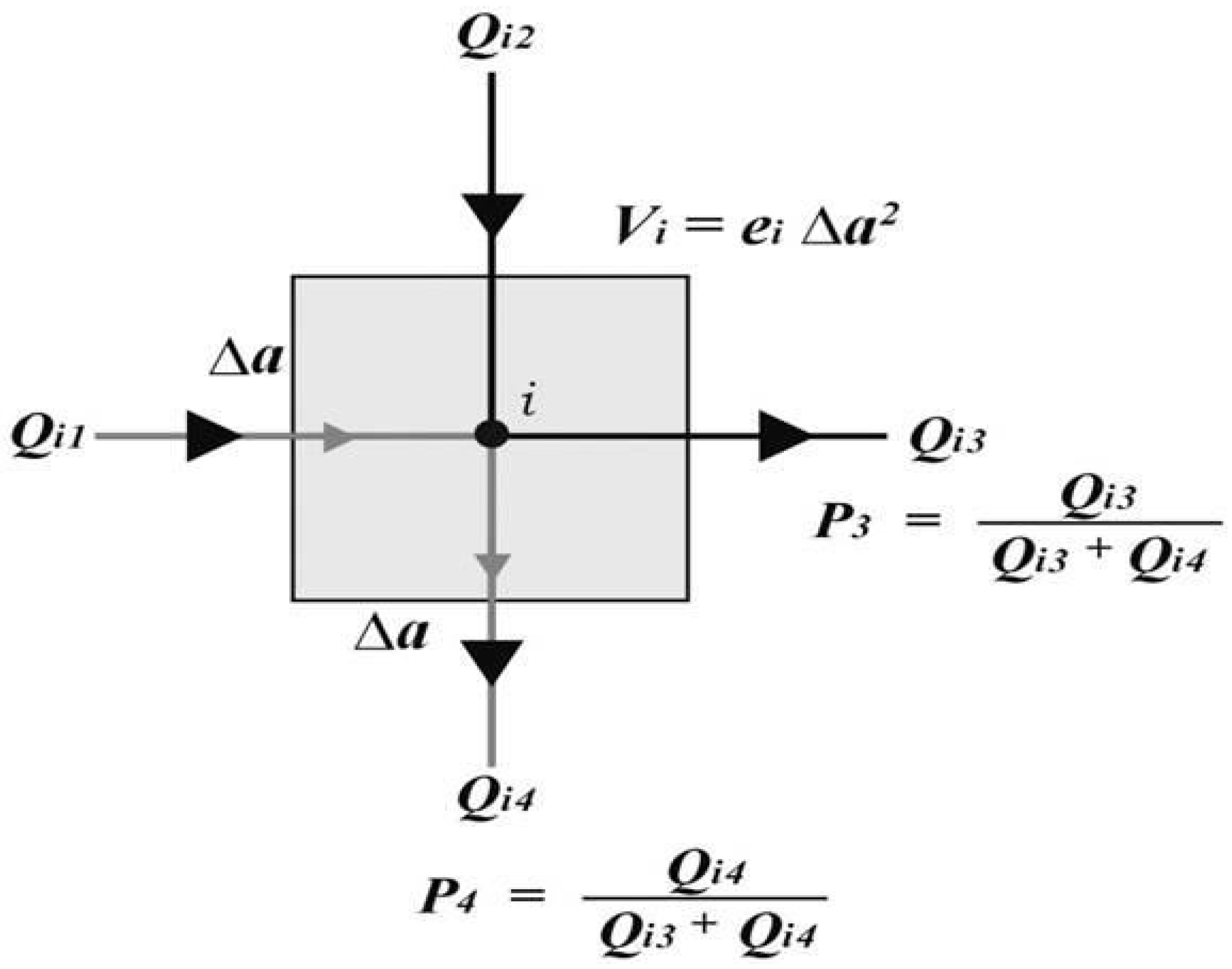
The RWPF model randomly extracts the location of solute particles at , and as a result, the mean residence time of solute particles is obtained between = 0 and . When solute particles being transported along the flow direction arrive at intersection , as shown in Figure 1, they select and move into any exit point based on the probability value and in proportion to the localized flow (P3 or P4 in Figure 1). As part of the element with aperture () and size , the residence time of solute particles is obtained by dividing the volume of the element () by the localized flow rate () as follows:
In addition, if the mean residence time of solute particles is presumed to be constant along the length of the fracture (), the actual residence time of solute particles can be calculated as follows:
where refers to the standard deviation of the normal distribution of distance travelled by solute particles, and refers to a random number in the range [−1, 1] that is generated by the law of normal distribution.
The residence time of a single solute particle calculated at each element from inflow boundary to outflow boundary is summed up to calculate the total residence time. This process applies to each of the solute particles, and the total residence time calculated for the solute particles is obtained in form of a breakthrough curve, thus indicating frequency of arrival of solute particles at the outflow point with passing time. In addition, in order to consider the retardation of solutes caused by adsorption as well as cracked walls and other factors, a retardation factor () is factored in to calculate the actual residence time of solute particles :
In this study, the matrix diffusion and molecular diffusion within fracture walls was not taken into consideration, and only spatial dispersion of solute transport caused by channeling phenomenon due to variable aperture distribution is considered.
3. Verification of RWPF Model
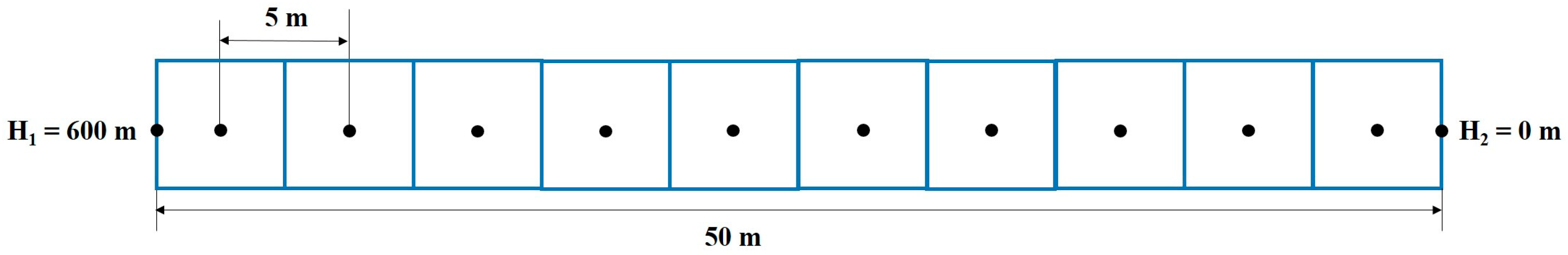
The one-dimensional channel system used to verify the RWPF model is shown in Figure 2. This channel system had a length of 50 m and consisted of 10 square-typed elements with a side length of 5 m. As boundary conditions, the hydraulic head value of = 600 m was imposed at the inflow boundary, and = 0 m at the outflow boundary.
The number of nodes was 12, and the distance between the nodes was 5 m. A total of 10,000 solute particles were injected into the left boundary , and the solute particles moving through the one-dimensional channel system arrived at the right boundary (Figure 2).
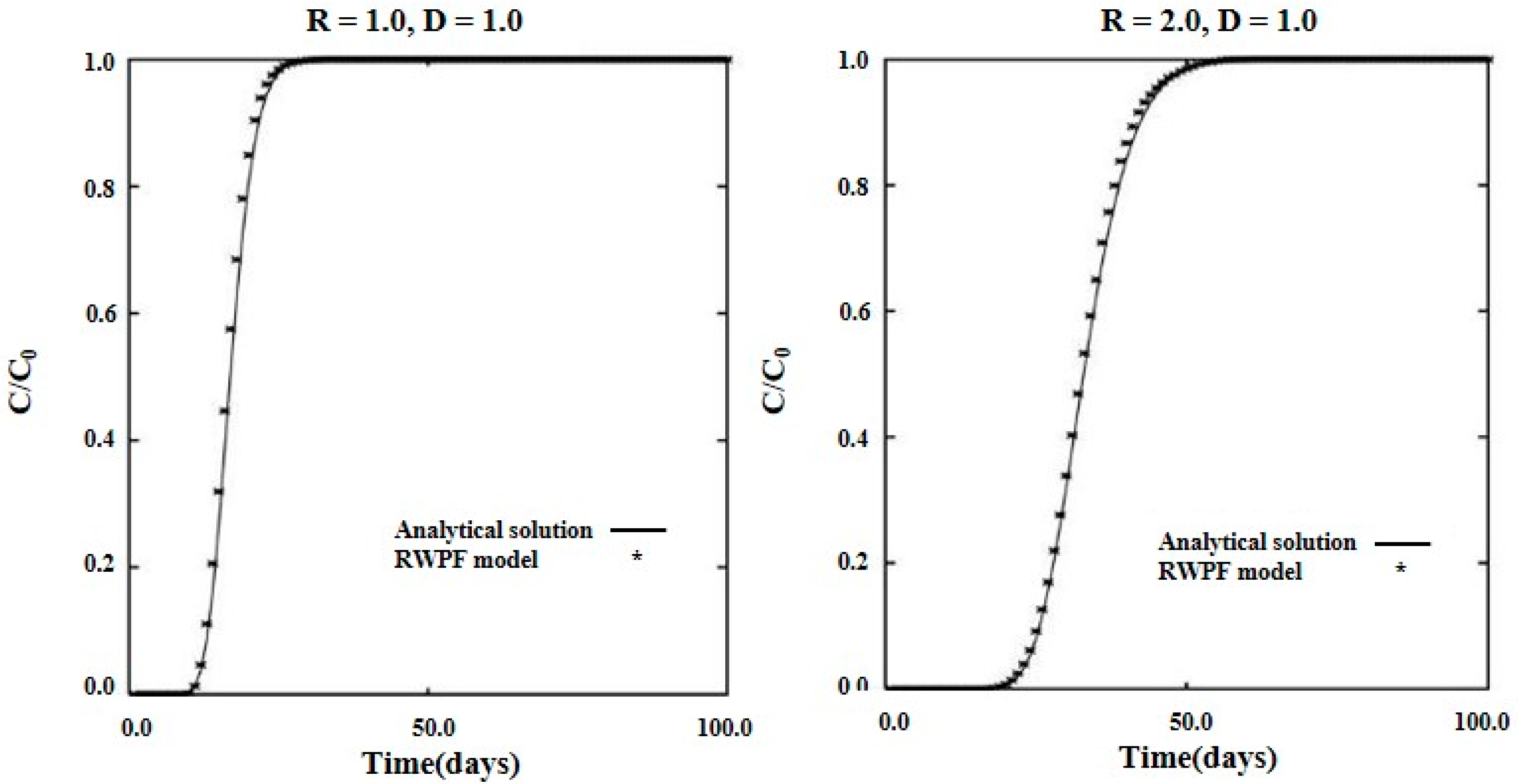
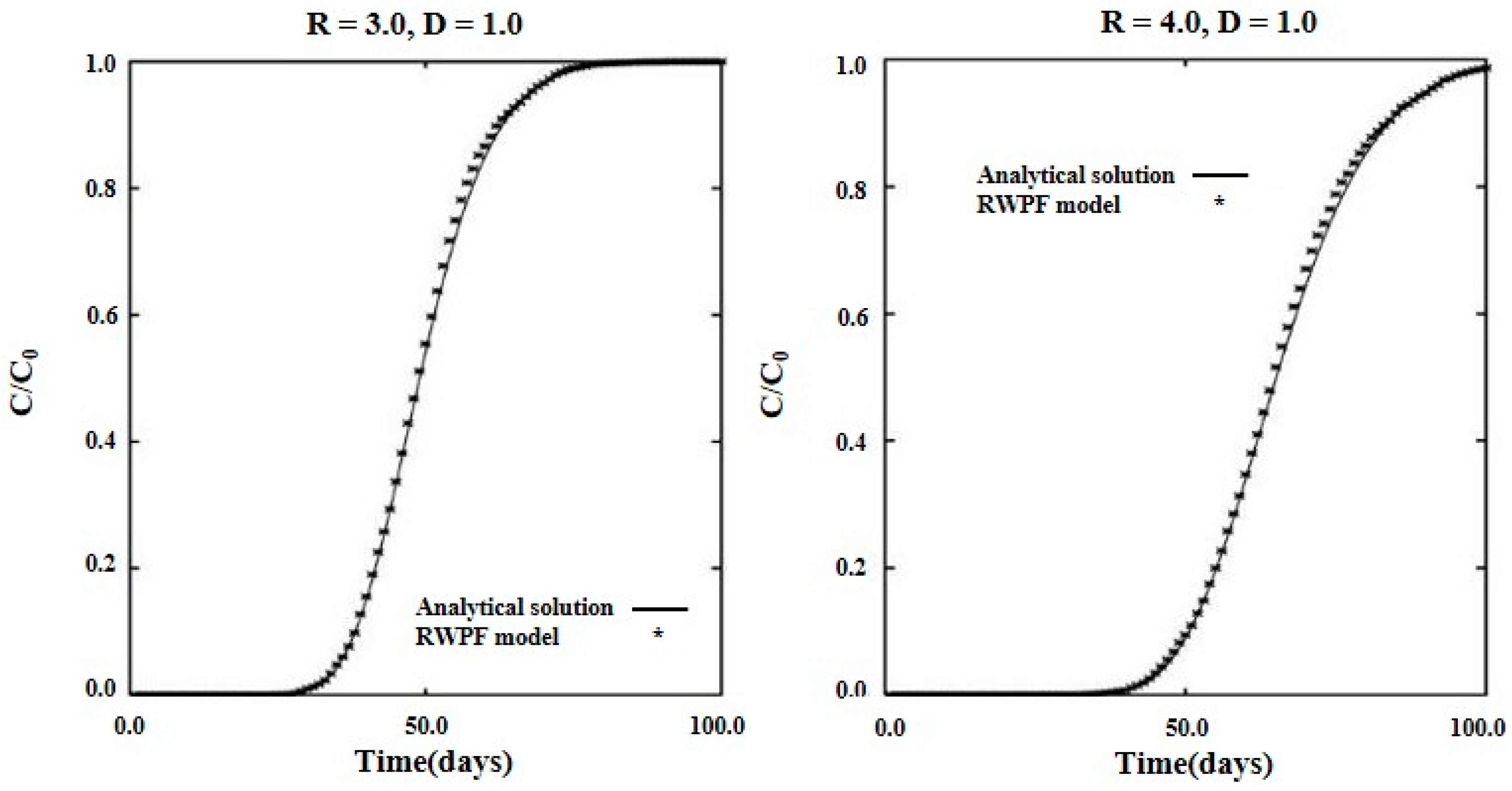
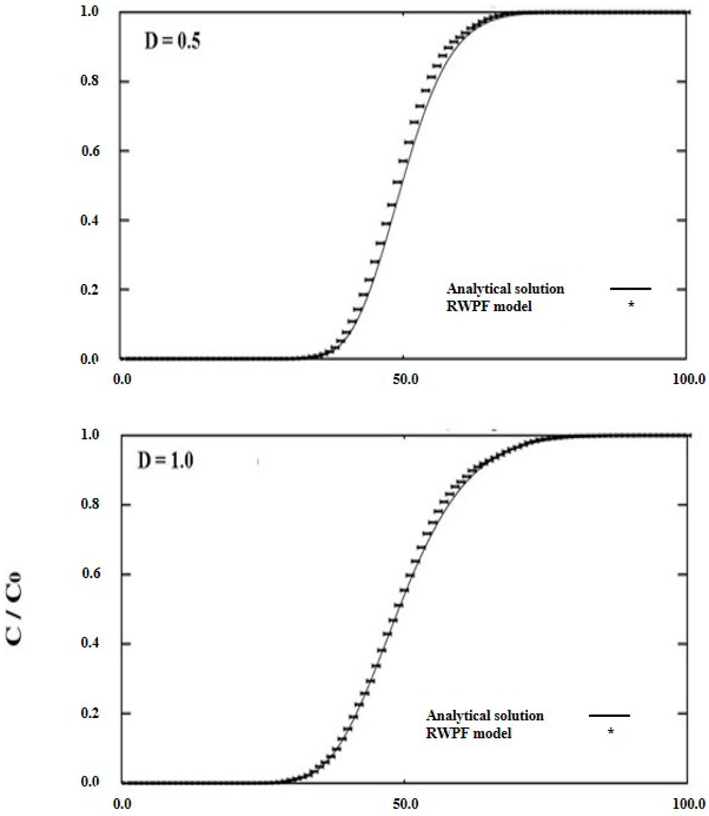
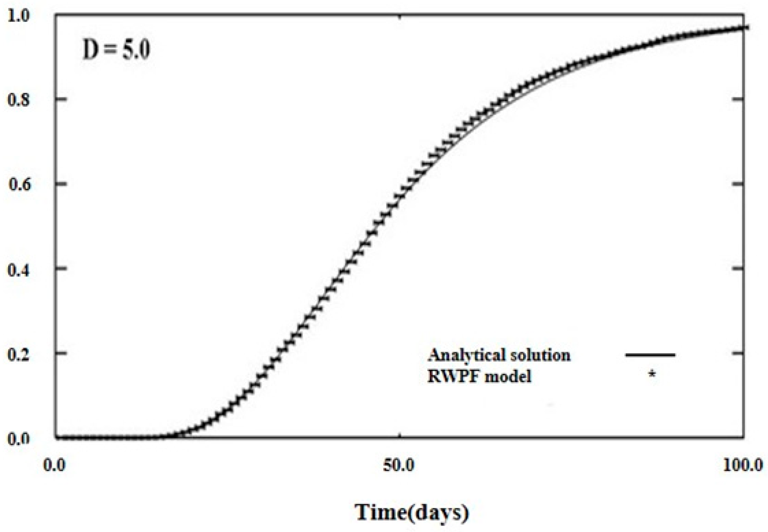
In this verification, the results of the simulation of solute transport based on retardation factor () and longitudinal dispersion factor () were compared with the analytical solution of the one-dimensional advection–dispersion equation in Equation (7) [19]. The applied values of were 1.0, 2.0, 3.0, and 4.0, and those of were 0.5, 1.0, and 5.0.
where [mg/m3] refers to the initial concentration, [m] to the length of the one-dimensional channel, [m/sec] to the velocity of solute particles moving along the direction of flow, and [m2/sec] to the longitudinal dispersion coefficient.
In this study, to compare analytical results from Equation (7) with numerical ones, it was assumed that was equivalent to , where was the number of solute particles arrived at boundary and the initial number of solute particles imposed at boundary . Figure 3 and Figure 4 show the comparison of the analytical solution with the simulation results of solute particle transport with and , respectively. As a result, it could be observed that simulation results of solute transport from the applied RWPF model agreed relatively well with analytical results in this study. In order to verify these comparisons more quantitatively, the RMSE (Root Mean Square Error) was estimated. The average of estimated RMSEs for four different values of was 0.0025 and 0.0032 for three different values of .
4. Solute Transport Simulation with Spatial Correlation Length and Effective Normal Stress
4.1. Simulation Condition
Simulations were performed to analyze the spatial behavior of solute transport within a single fracture in relation to spatial correlation length and mechanical effect of aperture distribution. In this study, 101 × 101 nodes were generated on the square surface of a fracture of size 100 m × 100 m, and it was assumed that the aperture distribution followed the law of log-normal distribution. In order to generate a spatially correlated aperture distribution, the turning bands algorithm and a geostatistical method was applied [20,21]. In this study, six correlation length ratios (correlation length /length of a single fracture , where the correlation length can be defined as a degree of the geometric correlation of apertures distributed within a given single fracture; length of a single fracture was fixed to 100 m) were considered. The considered correlation length ratios were: = 0.0 (no correlation), 0.1, 0.2, 0.3, 0.4, and 0.5. In addition, for mechanical effects, it was assumed that the effective normal stress was applied to a single fracture, with an increase in 5.0 MPa steps from 0.0 up to 35.0 MPa.
It was assumed that no retardation affecting solute particle transport—such as adsorption at fractured walls—existed (that is, = 1.0), and the value of was 1.0 m2/sec. The Monte–Carlo simulation (30 random numbers) was conducted for each value of , and applied for solute transport simulation. Analysis results presented are mean values.
Table 1 represents and closures used in solute transport simulation with mechanical effect. Results of the flow field used to simulate solute transport were reported by Jeong [20].
In order to simulate solute particle transport using RWPF numerically, first of all, flow velocity distributions for applied effective normal stresses and spatial correlation length ratios were required. The model used in this study consisted of two parts: the first was the flow model and the second the RWPF model. Solute particle simulation was conducted immediately after the flow simulation was finished under steady-state condition.
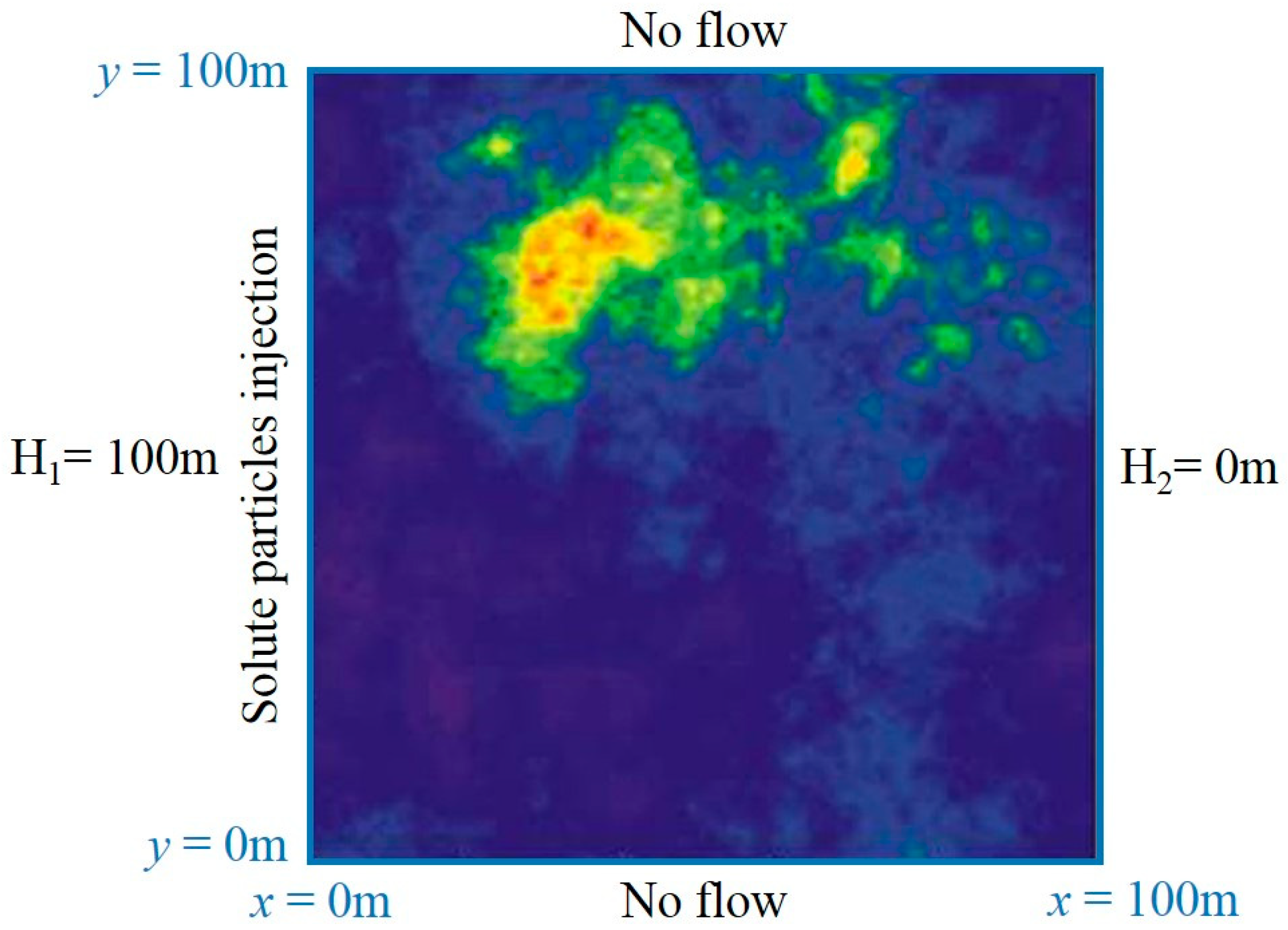
Figure 5 illustrates the square-typed single fracture and boundary conditions used in this study. The hydraulic head is prescribed as 100 m () at the left boundary and 0 m () at the right boundary. A total of 10,000 solute particles were injected along the boundary , and the solute particles were transported from the left to the right boundary. In this study, flow simulation results performed by Jeong [20] were for each level of effective normal stress and spatial correlation length ratio.
4.2. Breakthrough Curves and Mean Residence Time
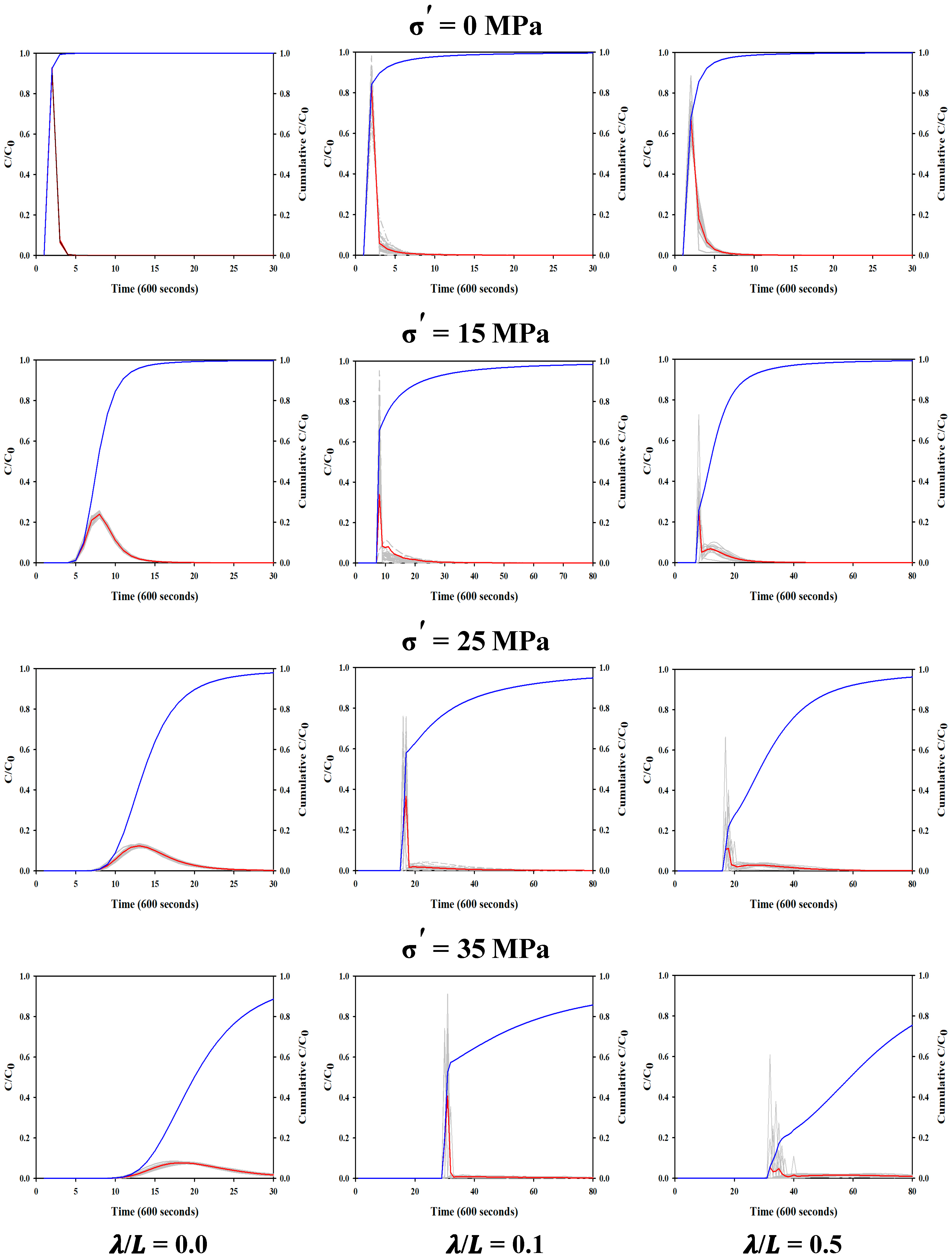
Figure 6 shows the variation of breakthrough curves of solutes based on and . The red line indicates the average of each breakthrough curve simulated using 30 random numbers, and the blue line indicates their cumulated breakthrough curve. When increased, the peak value of breakthrough curves tended to decrease gradually but the spatial dispersion increased. In case of no correlation, when increased, the time required to reach the peak value gradually decreased. These results were the same in case of , but once exceeded a certain value (15.0 MPa in this study), the time required to reach the peak value demonstrated a nearly constant trend. These results were delivered as solute particles that were transported through a nearly identical channel distribution owing to increase in contact surface after the value of exceeded 15.0 MPa.
Figure 7 shows the mean residence time of solutes with the values of and . The mean residence time remained almost constant when the values of increased along with to 10.0 MPa, but gradually increased from = 15.0 MPa. This was because increase in effective normal stress enlarged the contact surface within a single fracture, thereby increasing transport distance of solute particles.
Increasing tended to shorten the mean residence time largely because an increase in provided a flow-favorable channel [20], which then decreased the travel distance of solute particles. In case of no correlation, however, the mean residence time began to drastically increase from the point of = 15.0 MPa, which indicated that the aperture distribution with effective normal stress had an adverse effect on solute particle transport compared to that in case of spatial correlation length ratio.
4.3. Tortuosity of Solute Particles
In this study, an analysis of the spatial behavior of the particles that are transported through a curved channel with a varying aperture distribution or contact surface was conducted, and the travel routes of solute particles were determined. If particles passed through a single fracture having a varying aperture distribution or contact surface, they tended to travel via a curved route, as shown in Figure 8a. However, if solute particles traveled through a consistent aperture distribution across the entire single fracture, they showed a linear route, as shown in Figure 8b. The tortuosity of traveling solute particles could be obtained using the following equation [22]:
where [m] referred to the travel distance of the solute particles passing through a single fracture with varying aperture distribution; and [m] referred to the travel distance of the particles in a single fracture with a consistent aperture distribution, which was the same as the length of a single fracture.
Figure 9 illustrates the trajectories of solute particles passing through areas with relatively large localized flows based on an increasing effective normal stress for = 0.3. Increasing effective normal stress resulted in larger contact surfaces, which gradually increased the travel distance of the solute particles.
Figure 10 shows variations in tortuosity calculated using Equation (8) with and . Increase in resulted in a higher tortuosity because the increased effective normal stress resulted in larger contact surfaces and an increased travel distance of solute particles. In contrast, increase in spatial correlation length decreased the tortuosity because an increased spatial correlation length tended to generate an aperture distribution that is favorable to transport of solute particles. In addition, it could be observed that a higher effective normal stress generated wider differences in tortuosity based on correlation length. When values of 0.1 and 0.5 were compared, no significant difference was observed at = 0.0 MPa, but a difference of 0.7 and 1.3 was found at = 15.0 and 35.0 MPa, respectively. These results indicated that the aperture distribution with a longer correlation length was more favorable to transport of solute particles. In contrast to the correlation condition, tortuosity tended to increase along a nearly linear trend according to effective normal stress in case of no correlation, thus indicating that the aperture distribution that was favorable to transport of solute particles was not created.
4.4. Spatial Dispersion of Solute Particles
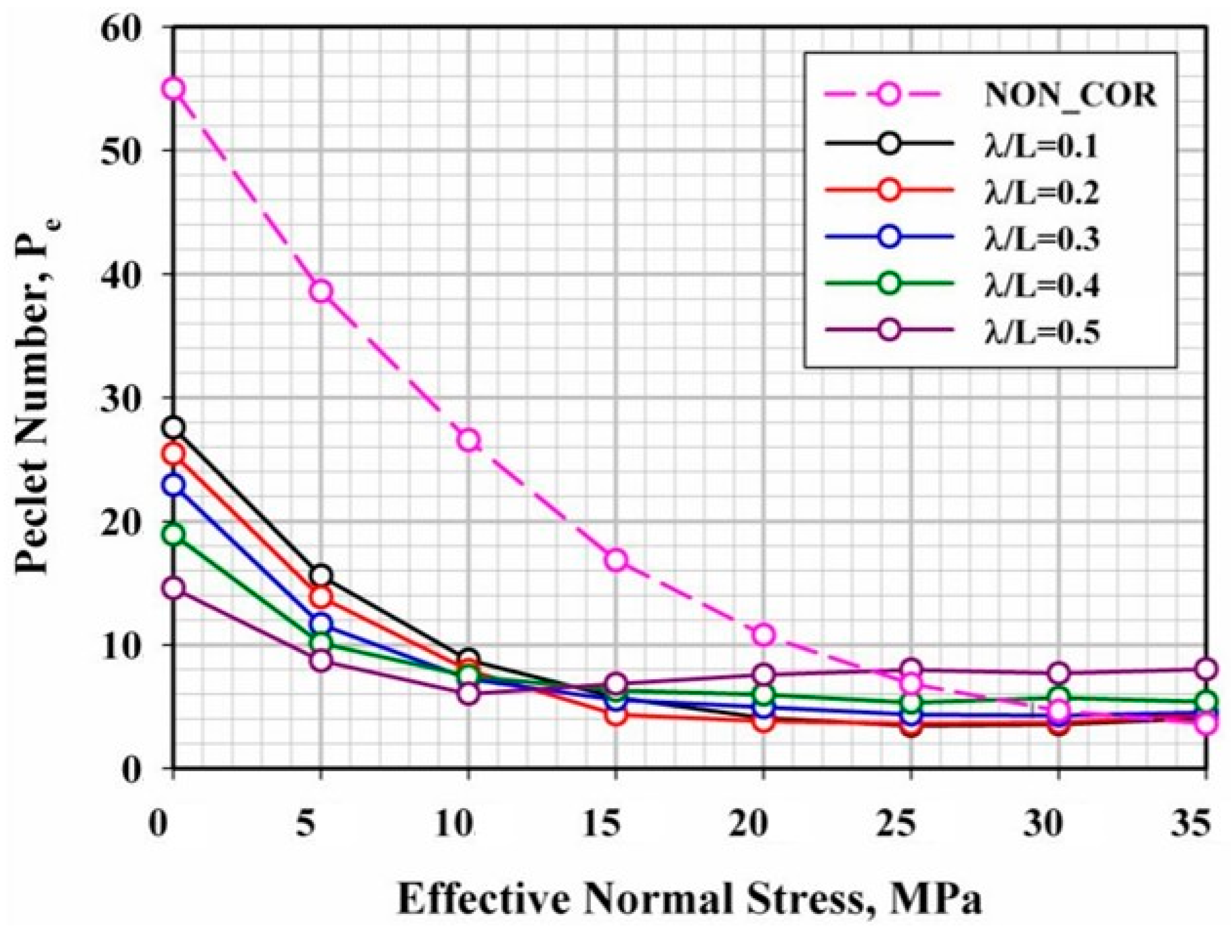
Peclet numbers can be defined as dimensionless numbers indicating the relationship between the rate of advection of solutes caused by flows and the rate of molecular diffusion. In this study, the Peclet numbers of solute particles for different values of and were estimated using the method suggested by Neretnieks et al. [23].
Figure 11 illustrates the variation in Peclet with and . The Peclet number was drastically reduced for all values until the point of = 10.0 MPa. However, after exceeded 10.0 MPa, the Peclet number tended to approach a certain constant value. This was because solute particles moved across the entire single fracture when values were small, but if values increased, solute particles moved through one or two major channels, as shown in Figure 5. In addition, while the Peclet number decreased as values increased until = 10.0 MPa, the Peclet number tended to approach a constant value at a faster pace when the values exceeded 10.0 MPa and values increased. This tendency reflected that as values increased, aperture distribution was more favorable to transport of solute particles. In case of no correlation, the Peclet number decreased exponentially when increased, in contrast to the case with correlation. When the value of was zero, the Peclet numbers varied from 14.6 ( = 0.5) to 27.6 ( = 0.1), according to the values of . Nerentnieks et al. [23] obtained Peclet numbers within the range of 9 and 27 in a laboratory experiment using granite samples with a diameter of 30 cm, and Moreno et al. [24] showed Peclet numbers varying from 9 to 80 for granite samples with a diameter of 27 cm. In a numerical experiment using a two-dimensional aperture model, Moreno et al. [12] suggested that the results of the experiment indicated Peclet numbers varying from 2 to 40 when effective normal stress increased. Furthermore, Thompson [13] used the fractal technique to observe a variation of Peclet numbers from 1 to 20 for solute transport within a single fracture with a spatially correlated aperture distribution. Thus, the results obtained in this study were consistent with results obtained from such indoor and numerical experiments.
4.5. Empirical Formula for Calculating Mean Residence Time of Solutes
The mean residence time of solute particles could be considered to be the actual mean residence time, thus reflecting effects of contact surface within a fracture and changing aperture distribution. This mean residence time was associated with the mean residence time that was calculated for a single fracture with a consistent aperture distribution:
where [m] referred to the average of aperture distribution purely provided for solute transport without considering ratios of contact surface based on effective normal stress, and indicated the average flow calculated using the cube law.
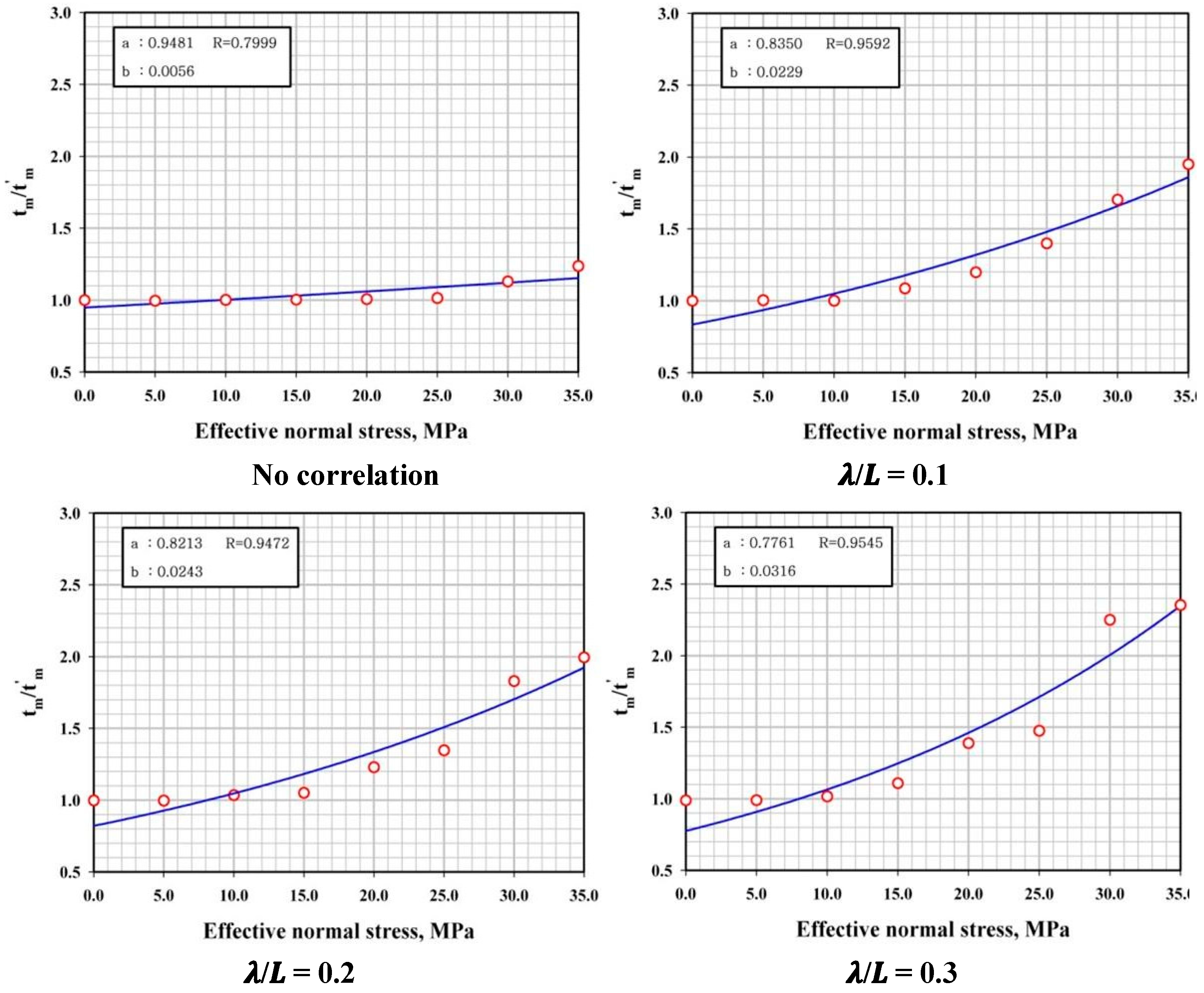
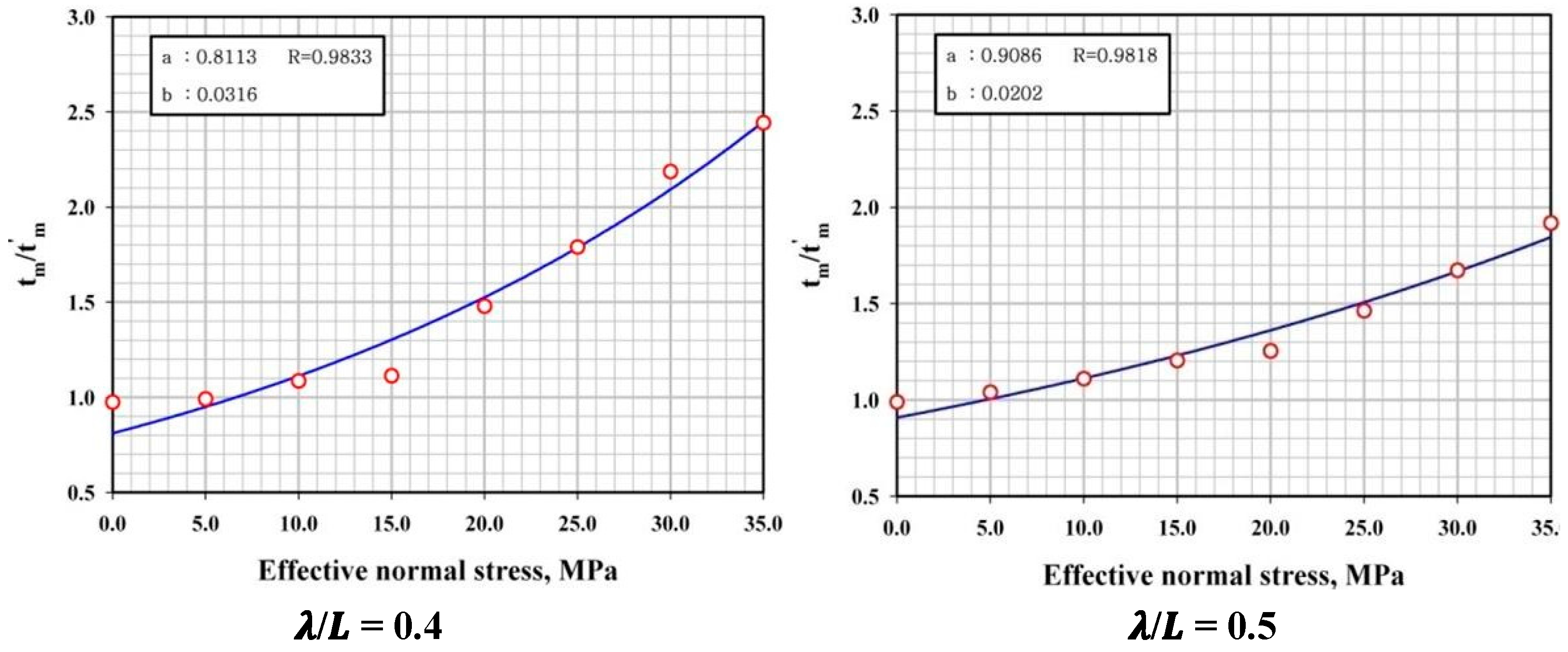
Figure 12 illustrates relations between and with , which showed an exponentially increasing tendency when increased. Based on these results, an empirical formula for and could be obtained as shown in Equation (10):
where and were parameters to be determined, and represented the inverse dimension of .
Equation (10) could be considered to analyze the relationship between the variation of mean residence time of solute particles and the applied effective normal stress in a single fracture with spatially correlated aperture distribution more quantitatively.
Table 2 presents the correlation coefficient () and the values of the constants and based on calculated from data of relations between and and from curve fitting of Equation (10). In general, tended to be 0.94 or higher in case of spatial correlation length. Therefore, Equation (10) reflected the simulated results of mean residence time of solutes well. In case of no correlation, however, the tendency of based on values of was slightly different from that in correlated condition, and the calculated value was 0.80, thus resulting in a slightly lower compatibility compared to that in correlation condition. The empirical formula of and suggested in this study was expected to be applicable for providing solute particle transport characteristics for individual fracture factors constituting fracture networks generated within a three-dimensional space, as in the study conducted by Nordqvist et al. [25].
The estimated parameters and did not show a tendency to increase or decrease apparently and regularly with variation of and λ/L and had a tendency to be more or less independent.
5. Conclusions
In this study, a numerical experiment was conducted to obtain characteristics of solute particle transport in a single fracture with apertures that were changed by spatial correlation length and effective normal stress. The results suggest that solute particle transport within a single fracture was significantly affected by the degree of spatial correlation length of aperture distribution and effective normal stress applied. With an increasing spatial correlation length, the mean residence time of solute particles were reduced and the tortuosity and Peclet numbers also decreased. This means that when the spatial correlation length increased, the aperture distribution within a single fracture became more favorable to transport of solute particles.
When the effective normal stress increased, however, the mean residence time and tortuosity tended to increase and the Peclet numbers decreased slightly. In particular, when the effective normal stress was 10.0 MPa or higher, the Peclet numbers tended to approach a certain constant value. This was because solute particles moved through one or two channels with relatively large localized flows owing to enlarged contact surfaces caused by increased effective stress.
Based on the results of solute particle transport simulation, this study also presents an exponential empirical formula to describe the relationship between effective normal stress and mean residence time of solute particles. This formula is expected to be used to estimate basic data for describing solute particle transport characteristics within individual fractures as analysis of the spatial behavior of solute transport in a three-dimensional fracture network was performed. However, the values of parameters a and b listed in Table 2 are limited to a single fracture of 100 m × 100 m. In order to become Equation (10) a more generalized formula, parameters a and b need to be determined with various sizes of single fractures.
Author Contributions
Conceptualization, Y.W.J. and W.C.J.; Methology and Simulations, W.C.J.; Model Development, W.C.J.; Result Analysis, Y.W.J.; Visualization, Y.W.J.; Project Administration, W.C.J.; Funding Acquisition, W.C.J.
Acknowledgments
This research was supported by a grant (code 17AWMP-B066761-05) from Advanced Water Management Research Program (AWMP) Program funded by Ministry of Land, Infrastructure and Transport of Korean government.
Conflicts of Interest
The authors declare no conflict of interest.
References
- Abelin, H.; Gidlund, J.; Neretnieks, I. Migration in a single fracture. Proc. Mater. Res. Soc. Symp. 1982, 11, 529–538. [Google Scholar] [CrossRef]
- Gale, J. Hydraulic behavior of rock joints. In Rock Joints; Barton, N., Stephansson, O., Eds.; Balkema: Rotterdam, The Netherlands, 1987; pp. 623–630. [Google Scholar]
- Gentier, S. Morphologie et Comportement Hydromécanique D’une Fracture Naturelle Dans un Granite sous Contrainte Normale: Étude Expérimentale et Théorique. Ph.D. Dissertation, University of Orleans, Orleans, France, 1986; pp. 1–350. [Google Scholar]
- Hakami, E.; Larsson, E. Aperture measurements and flow experiments on a single natural fracture. Int. J. Rock Mech. Min. Sci. Geomech. Abstr. 1996, 33, 395–404. [Google Scholar] [CrossRef]
- Haldeman, W.; Chuang, Y.; Rasmussen, T.; Evans, D. Laboratory analysis of fluid flow and solute transport through a fracture embedded in porous tuff. Water Resour. Res. 1985, 27, 53–65. [Google Scholar] [CrossRef]
- Pyrak-Nolte, L.; Myer, L.; Cook, N.; Witherspoon, R. Hydraulic and mechanical properties of natural fractures in low permeability rock. In Proceedings of 6th International Congress of Rock Mechanics; Balkema: Rotterdam, The Netherlands, 1987; pp. 789–798. [Google Scholar]
- Raven, K.; Gale, J. Water flow in a natural rock fracture as a function of stress and sample size. Int. J. Rock Mech. Min. Sci. Geomech. Abstr. 1985, 22, 251–261. [Google Scholar] [CrossRef]
- Witherspoon, P.; Wang, J.; Iwai, K.; Gale, J. Validity of cubic law for fluid flow in a deformable rock fracture. Water Resour. Res. 1980, 16, 1016–1024. [Google Scholar] [CrossRef]
- Brown, S. Fluid flow through rock joints: The effect of surface roughness. J. Geophys. Res. 1987, 92, 1337–1347. [Google Scholar] [CrossRef]
- Jeong, W.; Song, J. A numerical study on flow and transport in a rough fracture with self-affine fractal variable apertures. Energy Sources 2008, 30, 606–619. [Google Scholar] [CrossRef]
- LaBolle, E.M.; Fogg, G.E.; Tompson, A.F.B. Random-walk simulation of transport in heterogeneous porous media: Local mass-conservation problem and implementation methods. Water Resour. Res. 1996, 32, 583–593. [Google Scholar] [CrossRef]
- Moreno, L.; Tsang, C.; Tsang, Y.; Hale, F.; Neretnieks, I. Flow and tracer transport in a single fracture: A stochastic model and its relation to some field observations. Water Resour. Res. 1988, 24, 2033–2048. [Google Scholar] [CrossRef]
- Thompson, M. Numerical simulation of solute transport in rough fractures. J. Geophys. Res. 1991, 96, 6. [Google Scholar] [CrossRef]
- Tsang, Y.; Tsang, C.; Neretnieks, I.; Moreno, L. Flow and tracer transport in fractured media: A variable aperture channel model and its properties. Water Resour. Res. 1988, 24, 2049–2060. [Google Scholar] [CrossRef]
- Tsang, Y.; Tsang, C. Channel model of flow through fractured media. Water Resour. Res. 1987, 23, 467–479. [Google Scholar] [CrossRef]
- Ewing, P.; Jaynes, D. Issue in single-fracture transport modeling: Scales, algorithms and grid types. Water Resour. Res. 1995, 31, 303–312. [Google Scholar] [CrossRef]
- Vogler, D.; Settgast, R.; Annavarapu, C.; Madonna, C.; Bayer, P.; Amann, F. Experiments and simulations of fully hydro-mechanicallly coupled response of rough fractures exposed to high-pressure fluid injection. J. Geophys. Res. 2018, 123, 1186–1200. [Google Scholar] [CrossRef]
- Cacas, M.; Ledoux, E.; de Marsily, G.; Barbreau, A.; Calmels, P.; Gaillard, B.; Margrite, R. Modelling fracture flow with a discrete fracture network: Calibration and validation 2. The transport model. Water Resour. Res. 1990, 26, 491–500. [Google Scholar]
- Fetter, C. Contaminant Hydrogeology, 2nd ed.; Prentice Hall: New York, NY, USA, 1999; pp. 60–61. ISBN 0-13-751215-5. [Google Scholar]
- Jeong, W. Numerical Study on Behavior of groundwater flow in single rough fractures under mechanical effect. Groundwater 2017, 55, 38–50. [Google Scholar] [CrossRef] [PubMed]
- Matheron, G. The intrinsic random function and their applications. Adv. Appl. Prob. 1973, 5, 439–468. [Google Scholar] [CrossRef]
- Brown, S. Simple transport of fluid and electric current through a single fracture. J. Geophys. Res. 1989, 94, 9429–9438. [Google Scholar] [CrossRef]
- Neretnieks, I.; Eriksen, T.; Tahtien, P. Tracer movement in a single fissure in granitic rock: Some experimental results and their interpretation. Water Resour. Res. 1982, 18, 849–858. [Google Scholar] [CrossRef]
- Moreno, L.; Neretnieks, I.; Eriksen, T. Analysis of some laboratory tracer runs in natural fissures. Water Resour. Res. 1985, 21, 951–958. [Google Scholar] [CrossRef]
- Nordqvist, A.; Tsang, Y.; Tsang, C.; Dverstorp, B.; Anderson, J. A variable aperture fracture network model for flow and transport in fractured rocks. Water Resour. Res. 1992, 28, 1703–1713. [Google Scholar] [CrossRef]
Figure 1.
Solute particles’ selection of routes at intersection : black lines indicate the flow direction, and gray lines the particle routes. Random numbers exist between 0 and 1.
Figure 1.
Solute particles’ selection of routes at intersection : black lines indicate the flow direction, and gray lines the particle routes. Random numbers exist between 0 and 1.

Figure 2.
One-dimensional channel system applied to verify the RWPF (Random Walk Particle Following) model.
Figure 2.
One-dimensional channel system applied to verify the RWPF (Random Walk Particle Following) model.

Figure 3.
Comparison of simulation results of solute particle transport with with analytical solutions: the value of was fixed to 1.0 m2/sec.
Figure 3.
Comparison of simulation results of solute particle transport with with analytical solutions: the value of was fixed to 1.0 m2/sec.


Figure 4.
Comparison of simulation results of solute particle transport with with analytical solutions: the value of was fixed to 3.0.
Figure 4.
Comparison of simulation results of solute particle transport with with analytical solutions: the value of was fixed to 3.0.


Figure 5.
Square-typed single fracture and boundary conditions used in this study.

Figure 6.
Variations in breakthrough curves of solutes based on and . The red line refers to the average of breakthrough curves (bold gray lines) calculated through 30 random numbers, and the blue line to the accumulated breakthrough curves.
Figure 6.
Variations in breakthrough curves of solutes based on and . The red line refers to the average of breakthrough curves (bold gray lines) calculated through 30 random numbers, and the blue line to the accumulated breakthrough curves.

Figure 7.
Comparison of the mean residence time based on and .

Figure 8.
Travel trajectories of the solute particles for (a) varying aperture distribution and (b) consistent aperture distribution.
Figure 8.
Travel trajectories of the solute particles for (a) varying aperture distribution and (b) consistent aperture distribution.

Figure 9.
Trajectories of solute particles passing through a channel with relatively large localized flows when increased at = 0.3: (A) = 0.0 MPa, (B) = 15.0 MPa, and (C) = 35.0 MPa.
Figure 9.
Trajectories of solute particles passing through a channel with relatively large localized flows when increased at = 0.3: (A) = 0.0 MPa, (B) = 15.0 MPa, and (C) = 35.0 MPa.


Figure 10.
Comparison of tortuosity of solute particles with and .

Figure 11.
Comparison of Peclet numbers based on and .

Figure 12.
Relations between for and with .


Table 1.
Effective normal stresses () and closures used in this study [20].
Table 1.
Effective normal stresses () and closures used in this study [20].
| Effective Normal Stress | Closure |
|---|---|
| 0.0 | 0.0 |
| 5.0 | 139.0 |
| 10.0 | 212.0 |
| 15.0 | 258.0 |
| 20.0 | 289.0 |
| 25.0 | 312.0 |
| 30.0 | 329.0 |
| 35.0 | 342.0 |
Table 2.
Values of parameters and of Equation (10) determined based on .
| No Correlation | 0.1 | 0.2 | 0.3 | 0.4 | 0.5 | |
|---|---|---|---|---|---|---|
| a | 0.9481 | 0.8350 | 0.8213 | 0.7761 | 0.8113 | 0.9086 |
| b | 0.0056 | 0.0229 | 0.0243 | 0.0316 | 0.0316 | 0.0202 |
| CR | 0.7999 | 0.9592 | 0.9472 | 0.9545 | 0.9833 | 0.9818 |
© 2018 by the authors. Licensee MDPI, Basel, Switzerland. This article is an open access article distributed under the terms and conditions of the Creative Commons Attribution (CC BY) license (http://creativecommons.org/licenses/by/4.0/).
Share and Cite
MDPI and ACS Style
Jeong, Y.-W.; Jeong, W. Numerical Study of Spatial Behavior of Solute Particle Transport in Single Fracture with Variable Apertures. Water 2018, 10, 673. https://doi.org/10.3390/w10060673
AMA Style
Jeong Y-W, Jeong W. Numerical Study of Spatial Behavior of Solute Particle Transport in Single Fracture with Variable Apertures. Water. 2018; 10(6):673. https://doi.org/10.3390/w10060673
Chicago/Turabian StyleJeong, Yong-Wook, and Woochang Jeong. 2018. "Numerical Study of Spatial Behavior of Solute Particle Transport in Single Fracture with Variable Apertures" Water 10, no. 6: 673. https://doi.org/10.3390/w10060673
Note that from the first issue of 2016, this journal uses article numbers instead of page numbers. See further details here.