Evaluation of Thermal Stratification and Flow Field Reproduced by a Three-Dimensional Hydrodynamic Model in Lake Biwa, Japan


Division of Sustainable Energy and Environmental Engineering, Graduate School of Engineering, Osaka University, Yamada-oka 2-1 Suita, Osaka 565-0871, Japan
*
Author to whom correspondence should be addressed.
Water 2018, 10(1), 47; https://doi.org/10.3390/w10010047
Submission received: 12 October 2017
/
Revised: 5 January 2018
/
Accepted: 5 January 2018
/
Published: 9 January 2018
Abstract
:Water temperature near the surface of a lake increases with increasing air temperature, which results in stratification. The strength of stratification substantially influences the transport of water parcels from the surface to the bottom of a lake. In recent years, the stratification in Lake Biwa—the largest freshwater lake in Japan—has been stronger. However, it is difficult to reproduce the stratification well in the simulations. In the present study, we built a hydrodynamic model for the purpose of analyzing the structure of the stratification in detail. Using the model, we evaluated the reproducibility of the seasonal and annual changes of vertical water distribution and flow field in Lake Biwa from 2007 to 2011. The hydrodynamic model results show that the vertical water distribution approximately agrees with the field observations based on the statistical analysis. The seasonal change of thermal stratification is reasonably reproduced by the hydrodynamic model simulations. In the simulation, there are mainly two circulation flows at the surface layer of the lake. The first flows anticlockwise and the second flows clockwise in the northern part of Lake Biwa. In order to compensate for the surface water flow, the water under the thermocline sometimes flows in the opposite direction under each circulation flow.
1. Introduction
In a warm season, water temperature near the surface of a lake increases with increasing air temperature. This results in lake stratification. The thermocline disrupts the transport of substances such as dissolved oxygen between the surface layer and the layer under the thermocline. The period of stratification tends to be prolonged in lakes worldwide. Livingstone reported that in Lake Zurich (Switzerland), the rate of increase in water temperature at the surface was different from that in the deep layer from the 1950s to the 1990s due to climate change. Consequently, the thermal stability of the water rose by 20% and the period of the stratification was extended for two to three weeks [1]. Global warming may alter monomictic lakes, resulting in incomplete circulation [2]. For example, in Lake Constance (Germany), the overturning of water normally occurs once a year. However, with the prolonged increases in air temperature, observations show that overturning in winter has become incomplete in recent years [3]. This phenomenon may influence the ecosystem of the lake [4,5]. In some lakes, a lack of oxygen occurred in the deep layer during a stratified period because the thermocline disturbed the vertical mixing. The lack of oxygen can be offset during vertical mixing in winter, when ample amounts of oxygen are supplied to the bottom layer. In winter, the supply of oxygen in monomictic lakes influences the ecosystem in the lake. Global warming leads to prolonged periods of stratification in lakes [6]. Research using one-dimensional simulation models have predicted that, in moderate climates, global warming may lead to an oxygen deficit in the deep layers within a half century [7,8]. Previous studies have shown that thermal stability in lakes affects inter-annual variation of the bottom conditions during winter [9,10,11,12].
Other important factors which change the concentration of dissolved oxygen are internal waves and gravity currents. According to the research about Lake Kinneret (Israel), internal waves play a significant part in the transportation of materials in the bottom boundary layer [13]. Internal waves have also been studied in Lake Biwa by field observation [14], modal analysis [15], and numerical simulation [16,17]. Kitazawa et al. [18] showed that internal waves would affect the transportation of hypoxic waters in the bottom boundary layer. Additionally, gravity currents on the sloping boundary appeared to contribute to the restoration of the oxygen in the deep waters of Lake Biwa [19,20,21].
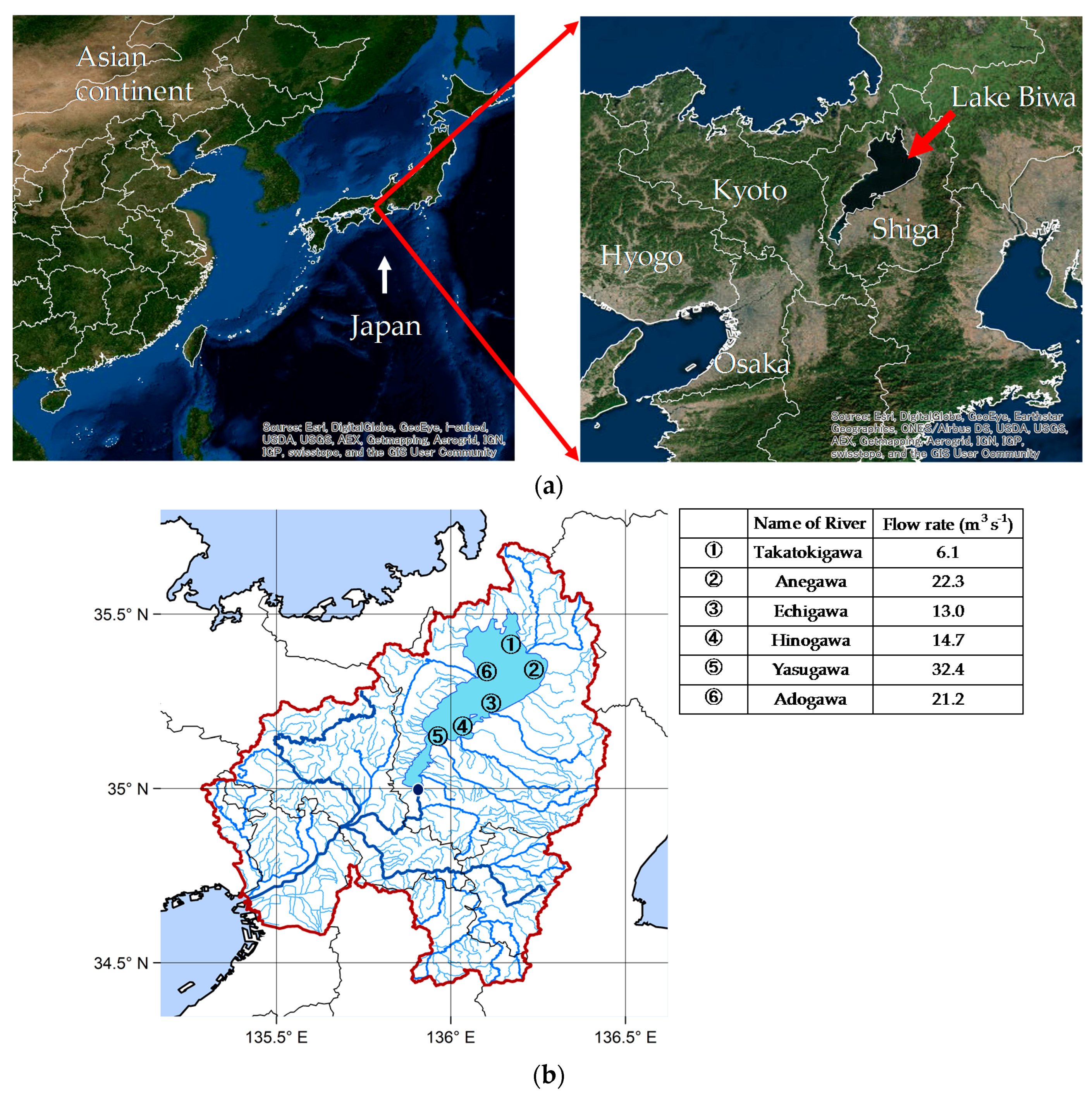
Lake Biwa is the largest freshwater lake in Japan, located in Shiga Prefecture (Figure 1a). It is approximately 63.5 km in length from north to south, and covers an area of 672 km2. Lake Biwa consists of two basins: a shallow south basin (mean depth: 4 m) and a deep north basin (mean depth: 44 m). The maximum width of Lake Biwa is 22.8 km, and its maximum depth is 103.6 m. It serves as a reservoir, providing drinking water for approximately 15 million people in Shiga and other surrounding prefectures.
Since the 1950s, the deterioration of Lake Biwa’s water quality has progressed [22]. In 1977, a large-scale freshwater red tide occurred in Lake Biwa. However, due to subsequent efforts to improve the lake’s water quality, the inflow of phosphorous has decreased. This has led to a decrease in eutrophication. After legislation to prevent eutrophication was enacted in 1981, the eutrophication had decreased. However, after the 1980s, low levels of dissolved oxygen under 2 mg/L in the bottom layer became evident. At this level, aquatic life cannot breathe naturally. The reason for the decrease in dissolved oxygen is believed to be the strengthening of stratification due to climate change in recent years [17]. Manifestations of climate change during the past thirty years, such as the decrease in precipitation, the rise in air temperature, and the decrease in wind speed, are considered causes of decreased dissolved oxygen in the bottom layer. In particular, the rise in air temperature and the decrease in wind speed weakens the mixing of the water mass; these may be the cause of low oxygenation in the bottom layer. However, the seasonal and inter-annual changes of stratification and the flow under the thermocline were not entirely clarified in the previous studies [17,18,23,24]. It is very difficult to reproduce the structure of stratification and flow field precisely in simulations which are controlled by the heat balance, the effect of the wind and river flows.
In the present study, we built a hydrodynamic model to evaluate the reproducibility of the seasonal and inter-annual changes of vertical distribution of water temperature and the water movement in Lake Biwa. The vertical distribution of water temperature and the structure of stratification in the simulation were investigated through comparison with the observations from 2007 to 2011. The period of model simulations in the present study is longer than in the previous studies [23,24]. In order to grasp the seasonal and annual change of structure of the stratification accurately, the grid size of the vertical direction is more detailed than in the previous studies [17,18,23,24]. Additionally, the development of the simulations for river and groundwater has progressed in recent years [25,26,27]. Therefore, the effect of the river inflows to Lake Biwa was taken into account by using the simulated data. Moreover, the flow field from the surface layer to the bottom layer was analyzed in the present study. In the near future, we will investigate if the structure of the stratification changes due to the variations in air temperature, wind speed, and precipitation by modifying the meteorological conditions in the numerical experiments. Therefore, this research is the first step in validating the model.
2. Hydrodynamic Model in Lake Biwa
2.1. Calculation Domain
Figure 1a shows the location of Lake Biwa in Japan, and Figure 1b shows the location of its rivers’ inflows and outflows. Water depth in Lake Biwa is shown in Figure 1c. The calculation domain is latticed by the structured grid. The horizontal model domain is 36 km by 65.5 km, with a grid size of 500 m. The vertical domain depth is 107.5 m. The vertical layer thickness is 0.5 m from the surface to 20 m in depth; it varies from 0.5 to 2.5 m as the depth increases vertically by 0.1 m increments. This is to more accurately reproduce the change of water temperature in the surface layer, as compared to other models in previous studies. A staggered grid system is adopted to calculate the water temperature, density, pressure, and velocity within the model domains.
2.2. Hydrodynamic Model
According to Akitomo et al. [23] and Kitazawa and Kumagai [24], the governing equations consist of the momentum equation with Boussinesq approximation, the hydrostatic equation, the continuity equation, and the conservation equation for temperature. The governing equations are described in the Cartesian coordinate system as demonstrated below. The origin of the coordinate axes is in the southwestern edge of the domain on the horizontal plane. The x and y axes are set to west–east and south–north directions, respectively, and the z axis directs upward.
The momentum equations (x, y direction) are:
the hydrostatic equation is:
the continuity equation is:
the conservation equation for temperature is:
the density of water is calculated using:
where , , and are the , , and components of current velocity (m·s−1), is the water temperature (), is the pressure (N·m−2), is the density of water (kg·m−3), is the reference density of water (103·kg·m−3), is the acceleration due to gravity (9.8 m·s−2), is the Coriolis parameter (8.34 × 10⁻⁵·s−1 corresponding to 35° N), is the horizontal eddy viscosity coefficient for momentum equations (1.0 m2·s−1), is the horizontal eddy diffusivity coefficient (1.0 m2·s−1), is the vertical eddy viscosity coefficient (m2·s−1) for momentum equations, and is the vertical eddy diffusivity coefficient (m2·s−1). The horizontal eddy viscosity and diffusivity coefficients (1.0 m2·s−1) were chosen as the constant values [23].
The governing equations were discretized using the finite volume method. The first-order Euler method was employed for the time discretization, the second-order central discretization method was employed for the diffusion term, and the first-order upwind method was employed for the convection term. The time increment is 10 s.
In summer, a thermocline is typically formed at depths from 10 to 30 m. This thermocline suppresses the vertical transport of momentum and heat. To take this effect into account, the parameter values of vertical eddy viscosity and diffusivity are estimated by using the Richardson number [24,25,26]. The Richardson number is a dimensionless number that expresses the ratio of the buoyancy term to the flow gradient term and is calculated by:
where is the horizontal current velocity (m·s−1). The vertical eddy viscosity and diffusivity are respectively calculated using:
and
There are many papers on hydrodynamic simulations of lakes using the higher order turbulence schemes [16,20,28,29,30]. However, according to Ishizuka et al. [31], there were no significant differences in the vertical water distribution among the results of the turbulence scheme with Equations (7)–(9), the Mellor–Yamada turbulence model [32], and the k-ε model [33]. Because it takes less time to calculate the vertical eddy diffusivity and viscosity compared to calculating the transport equations in the other two models, this model is applied to the hydrodynamic model. The method of turbulence model described by Equations (7)–(9) was originally derived by Munk and Anderson [34], and Webb [35].
We built the hydrodynamic model based on these governing equations. The model was written in Fortran. The numerical simulation was carried out during the period from 1 April 2007 to 31 March 2012. The spin-up period was from 1 April 2006 to 31 March 2007.
2.3. Initial Conditions
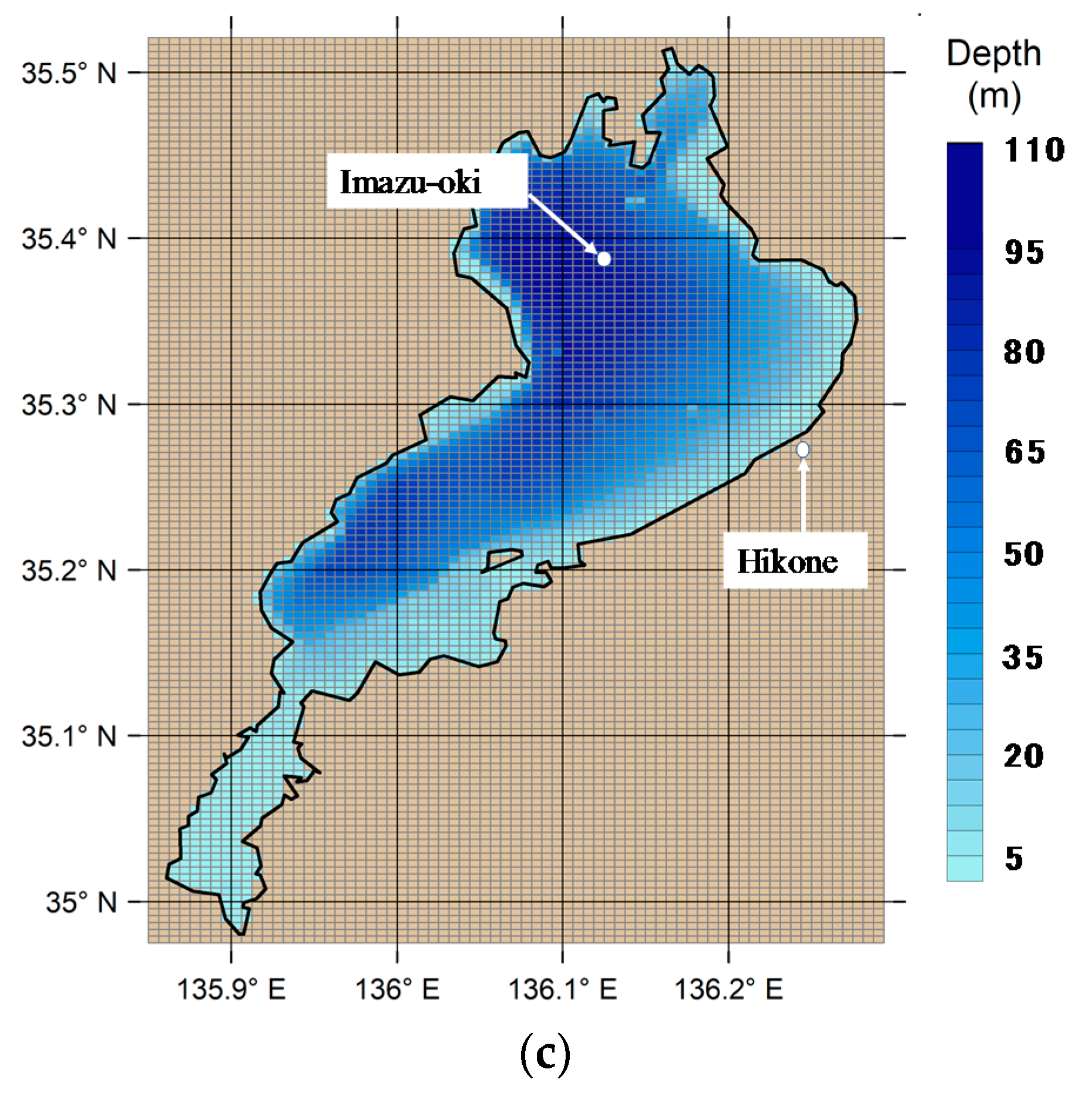
For the initial condition, the current velocity was set to be 0 m·s−1, and the initial water temperature was derived from linear interpolation of observed vertical profile data on 20 March and 10 April 2006. The observations were conducted by the Lake Biwa Environmental Research Institute twice a month at the monitoring point in Imazu-oki (35°23′41″ N, 136°07′57″ E), the depth of which was 0.5 m, 5 m, 10 m, 15 m, 20 m, 30 m, 40 m, 60 m, 80 m, and approximately 90 m.
2.4. Boundary Conditions
The boundary conditions for the velocity at the surface of the lake are given by the following equations by taking the wind stress into account:
where and are the surface wind frictional stresses calculated using
where is the density of air (kg·m−3), is the wind frictional constant (−), is the wind speed from a height of 10 m above the surface (m·s−1), and and are the and components of wind velocity (m·s−1), respectively.
The water surface elevation is calculated using:
The boundary condition for the gradient of water temperature is calculated by the integration of short-wave solar radiation, latent heat flux, sensible heat flux, and net long-wave radiation, which is then divided by the density of water, specific heat of water, and vertical eddy diffusivity.
The heat flux through the water surface consists of short-wave solar radiation (), latent heat flux (Ql), sensible heat flux (Qs), and net long-wave radiation (Lnet). According to Kondo [36], the heat balance equation on the water surface is given by:
where is specific heat of water ( (J·kg−1·K−1)).
Short-wave solar radiation is calculated using:
where (W·m−2) is the observed global solar radiation and ref stands for albedo. Albedo is defined as the ratio of irradiance reflected to the irradiance received by a surface. ref is around 0.03 when the surface maintains a fixed position, however it reaches 0.1 when the wind blows. ref was assumed to be 0.07 (−). Some of the short-wave solar radiation is absorbed by the surface water, while other intrudes into deep waters.
Assuming that the intensity of the short-wave-radiation decreases exponentially with the distance from the water surface, the intensity of the short-wave radiation at the water depth of z (m) can be calculated as:
where is water depth (m), is short-wave solar radiation at the water surface (W·m−2), and is the intensity of the short-wave solar radiation at the depth of z (W·m−2).
Latent heat flux and sensible heat flux are formulated by bulk formula according to Kondo [37] and Hirose et al. [38].
Latent heat flux (Ql) is estimated by:
where is the bulk constant coefficient of latent heat with 1.2 × 10⁻³ (−) as the constant value. is latent heat of evaporation (2.45 × 10⁶ (−)).
is saturation specific humidity (−) and is specific humidity (−). These values are calculated by:
where is the saturated vapor pressure (hPa), is atmospheric vapor pressure (hPa), is atmospheric pressure (hPa), and is water temperature at the surface of the lake.
Sensible heat flux (Qs) is estimated by:
where is the specific heat of air (1.01 × 10³ (J·kg−1·K−1)), is the bulk constant coefficient of sensible heat (1.2 × 10⁻³ (−)), is atmospheric temperature, and is water temperature at the surface of the lake.
Net long-wave radiation (Lnet) is calculated using:
where emissivity is 0.98 (−), Stefan–Boltzmann constant is 5.67 × 10⁻⁸ (W·m−2·K−4), surface reflectivity is 0.2 (−), the amount of cloud is in the range from 0 to 100 (%), and the correction coefficient is ().
The no-slip condition is imposed at the bottom and on the side walls. The normal gradients of water temperature are also zero, so there is thermal insulation.
2.4.1. Meteorological Conditions
Air temperature, atmospheric pressure, wind direction and speed, and relative humidity over Lake Biwa were derived from the Grid Point Value, which in turn is derived from the Meso-Scale Model of the Japan Meteorological Agency (GPV MSM). GPV MSM data has a spatial resolution of 0.0625° longitude by 0.05° latitude (approximately 5 km) and a temporal resolution of one hour. The data was horizontally interpolated into each surface mesh of the hydrodynamic model. Solar radiation was derived from hourly observation data at the Hikone Local Meteorological Observatory (35°16′30″ N, 136°14′36″ E), as shown in Figure 1c. Solar radiation was assumed to be horizontally uniform over the lake. The time series of air temperature, short-wave solar radiation, and wind velocity observed at Hikone for using the initial conditions are shown in Figure 2a–c.
2.4.2. River Conditions
In taking the effect of the river inflows to Lake Biwa into account, the simulated data instead of the field observations were given as boundary conditions. The water temperature and volume which were calculated by a hydrological model were interpolated each day for fifty-six rivers. The location of six main rivers and the annual mean river inflow rates are shown in Figure 1b. The total mean amount of annual river inflow rate is 177.5 m3·s−1. The amount for six main rivers accounts for about 60% of the total inflow. The only outflowing river, Setagawa, is located at the southern-most part of Lake Biwa, as shown in the blue point of Figure 1b. The data of the river inflow was updated in detail every day for the analysis. The boundary conditions for the water volume and temperature associated with each river’s inflow and outflow were calculated using the hydrological model [39].
2.5. The Method of Evaluation of the Reproducibility of the Three-Dimensional Hydrodynamic Model
The hydrodynamic model of Lake Biwa was validated by comparing the model results with the observed data. Simulated water temperatures were compared with field observations from the monitoring point in Imazu-oki. As statistical indicators, the correlation coefficient () between observed and calculated values, mean absolute error (MAE), and mean bias (MB) were used and were calculated, respectively, using:
where is observed water temperature at each point twice a month, is simulated water temperature at each point twice a month, and is the number of samples.
Statistical indexes between observed data and simulated data were calculated at the ten points from a depth of 0.5 m to 90 m, twice a month, at the same place and time, from 2007 to 2012 for five years. For calculating the statistical indexes in the surface layer, thermocline, and bottom layer, the data at a depth of 0.5 m, 20 m, and 90 m was used, respectively. For statistical indexes in the thermocline, the data around the center of the thermocline was chosen. The data in each year (taken from April to the following March) was divided by intervals of three months. These four periods were defined as four seasons (i.e., spring, summer, autumn, and winter). The annual index was calculated by using data from April to the following March.
3. Results and Discussions
3.1. Comparison between Model Results and Observations
3.1.1. Evaluation of the Reproducibility of the Three-Dimensional Hydrodynamic Model
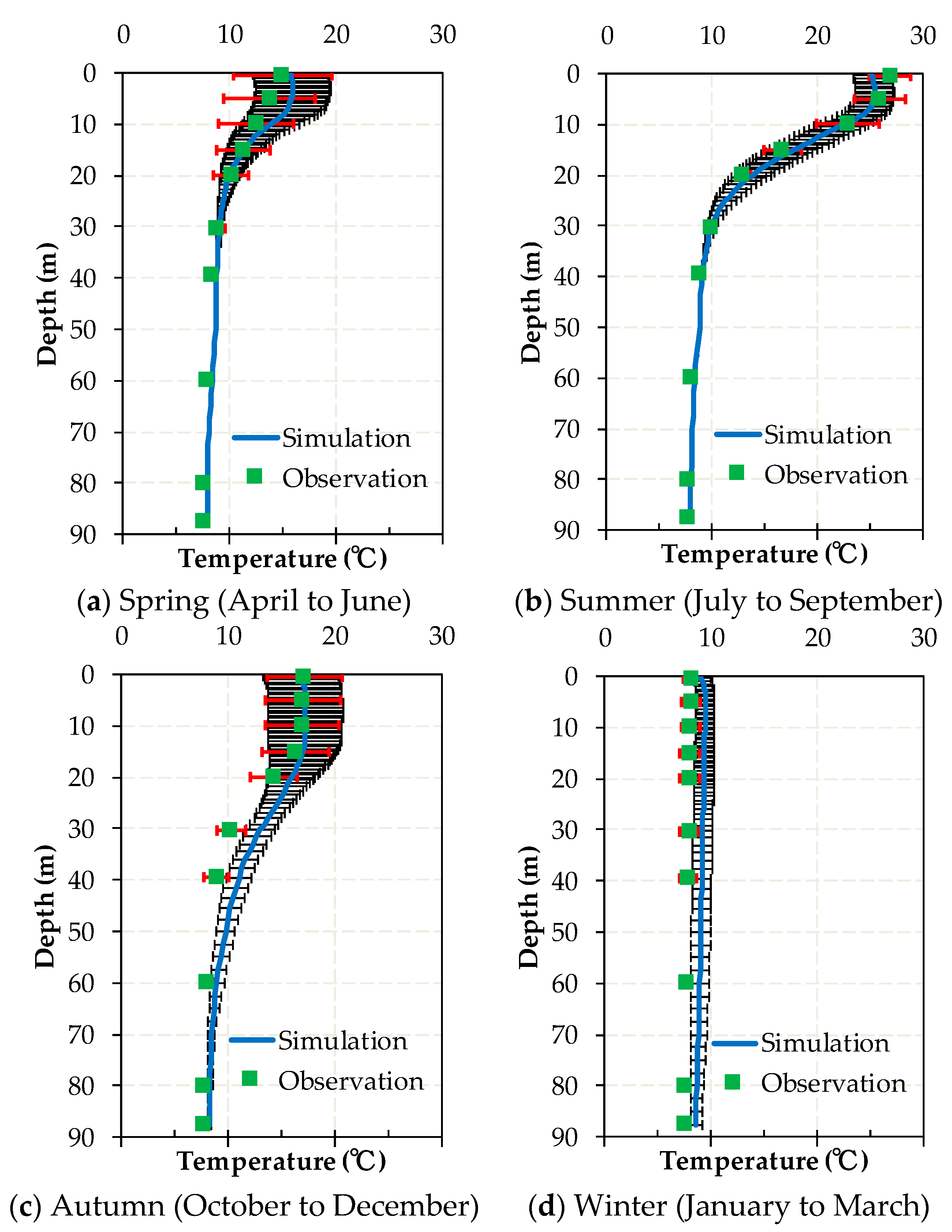
The correlation coefficients are higher than 0.9 from spring to autumn and higher than 0.8 in winter, as shown in Table 1. In winter, the correlation coefficients are low due to the lower water temperature in winter compared to that in summer, as shown in Figure 3. The gradients of simulated and observed water temperatures of winter are interchangeable because the water temperature of all layers become uniform. Table 1 shows that MAE in every season are lower than 1.3 °C. MB is also under approximately 1.3 °C. The difference between MAE and MB becomes similar in winter, showing that the water temperatures of all layers have some discrepancies between the simulation and observation. As the water temperatures in autumn and winter are slightly higher than the observed values, it is indicated that the cooling flux is not transferred to the deep layer. There is a possible reason that the effect of the wind also plays a more important role in transferring the cooling flux in cooling seasons. Hence, the vertical mixing is difficult to reproduce well using the model. However, the rate of the error is small in other seasons, which shows that the model results agree well with the observation data. We also investigated the differences of change in the water temperature at various depths. Figure 3 represents the annual mean value and standard deviation of the vertical distribution of water temperature for every three months from 2007 to 2012. The simulated water temperature in the surface layer is slightly higher than the observed temperature in spring. In autumn, the simulated water temperature is slightly lower than the observed temperature. However, according to the correlation coefficients in the surface layer, the trend of surface temperature is well reproduced. In the thermocline, the simulated water temperature is higher than the observed temperature from summer to winter (Figure 3). MAE during that period is higher than in spring; this indicates that during the period of the stratification, the vertical distribution of water temperature in the thermocline is difficult to reproduce. At a depth of 30–40 m in autumn, the discrepancy between the simulated water temperature and the observed temperature may be due to not calculating the vertical diffusivity based on the effect of the wind stress. As described above, in order to match the simulated water temperature to the observation, it may be necessary to more precisely account for the wind stress under neutral or stratified conditions.
In the bottom layer, the simulated water temperature is almost the same as the observed value all year. However, in winter, it is higher than the observed temperature (Figure 3). Furthermore, according to Figure 3, the correlation coefficients are very low in the bottom layer because the deviation of the water temperature in this layer is smaller than that of the surface layer.
3.1.2. Water Temperature from the Surface to the Bottom Layers
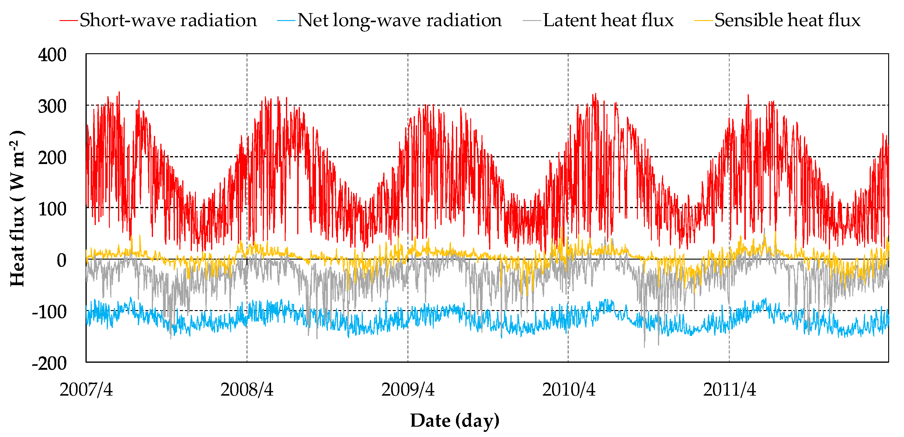
Figure 4 shows a time series of short-wave radiation, net long-wave radiation, latent heat flux, and sensible heat flux at the monitoring point in Imazu-oki from 2007 to 2012. The largest amount of cooling flux is evident in net long-wave radiation, with latent heat flux being greater than net long-wave radiation during summer. In summer, sensible heat flux decreases because of the small difference between water temperature and air temperature. However, in winter, the cooling components of sensible heat flux is high because water temperature is higher than air temperature. The loss of the latent heat flux due to evaporation is also influential. Therefore, the pattern of cooling flux plays an important role in vertical mixing.
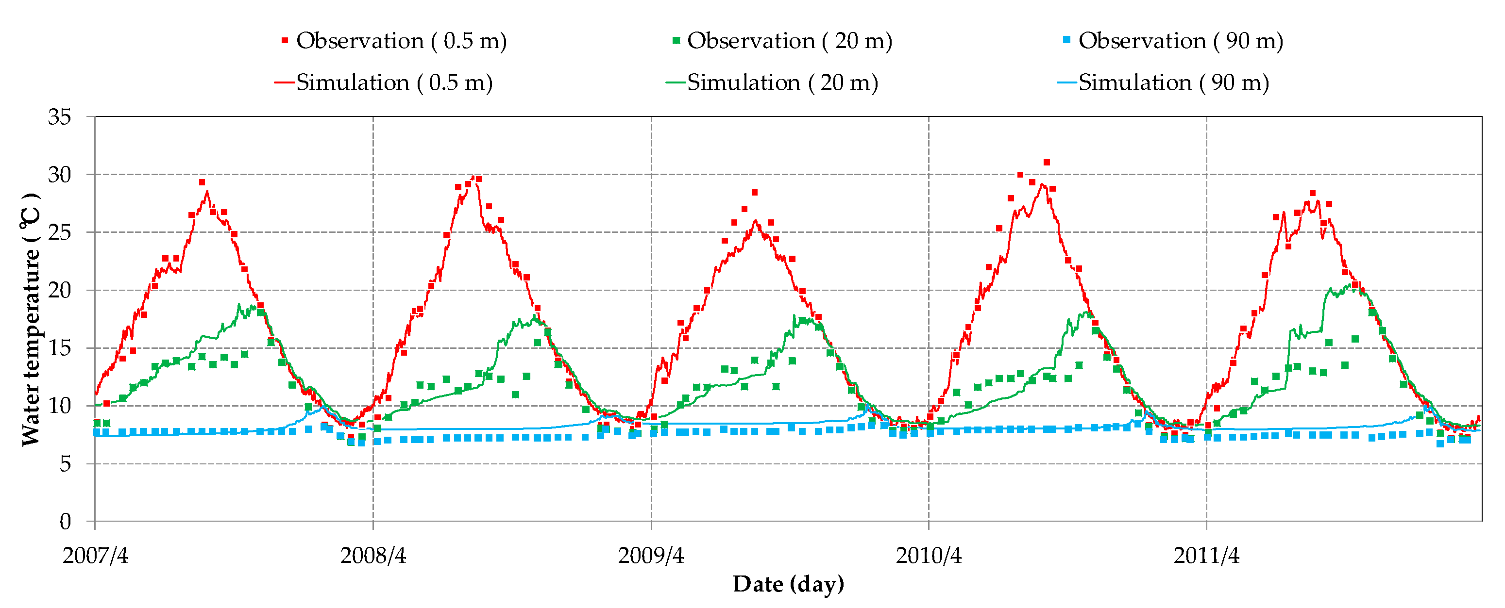
Figure 5 shows a comparison of observed and simulated water temperatures at depths of 0.5 m, 20 m, and 90 m at the monitoring point in Imazu-oki, as previously described. The simulated water temperature in the surface layer is lower than the observed temperature in summer. The cause of this is inferred to be a lack of heat flux during the summer. Therefore, the formulation of the heat balance should be considered in more detail. In actuality, the amount of short-wave radiation above the surface of the lake is more than that on land during the summer. As for the thermocline, the simulated water temperature is higher than the observed value from autumn to winter (Figure 5).
In the bottom layer, the simulated water temperature coincides with the observed temperature all the year around, although in winter it is higher than the observed value. From autumn to winter, the air temperature lowers and cools the water temperature in the surface layer downward. Eventually, the water in the surface layer reaches the lower layers, and the temperature of all layers becomes the same due to overturning. Furthermore, in the middle of winter, the air temperature is much lower than the water temperature of all layers, so the water temperature in the bottom layer is cooled to lower than that of the summer. The water temperature of all layers is controlled by the air temperature in the middle of winter each year. Therefore, it is essential that the simulated water temperature in winter is matched reasonably well with the observations.
3.2. General Model Results
3.2.1. Seasonal Change of the Structure of Stratification at the Monitoring Point in Imazu-Oki
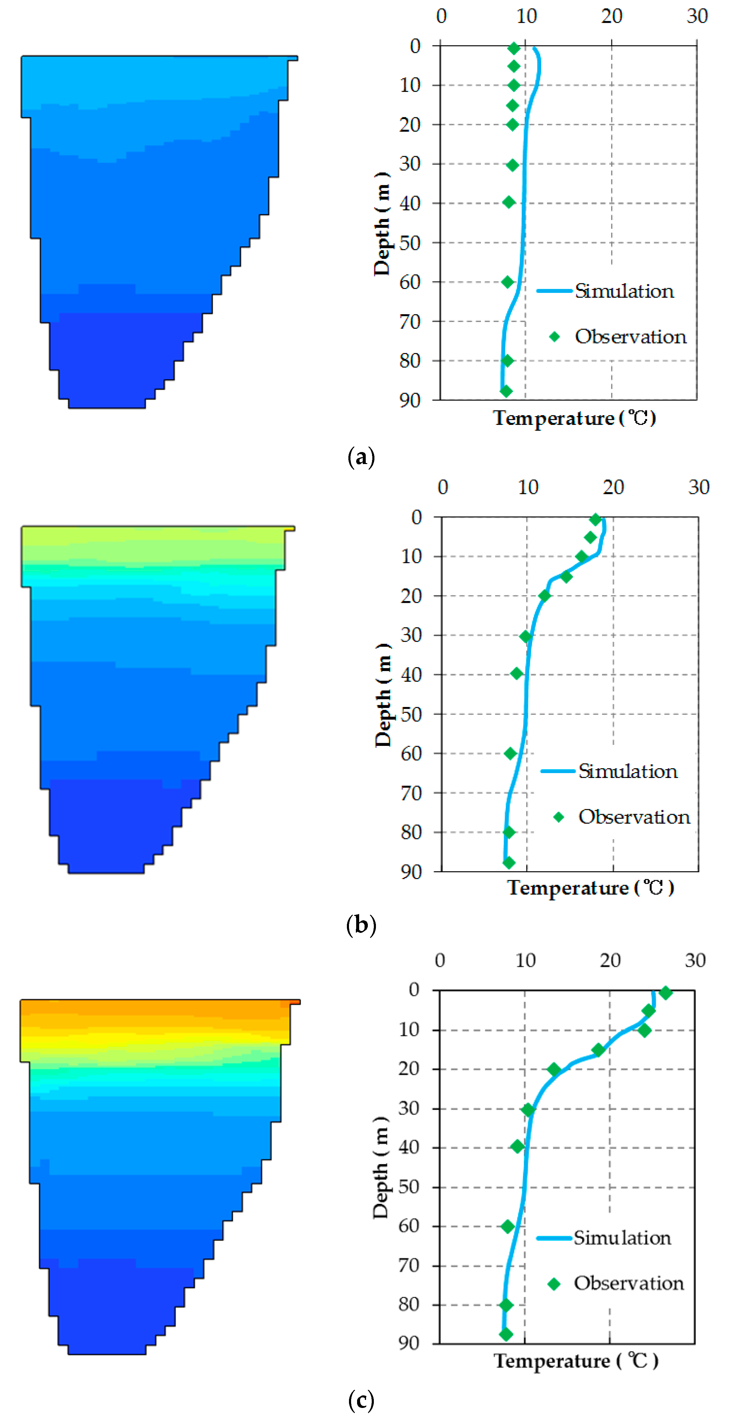
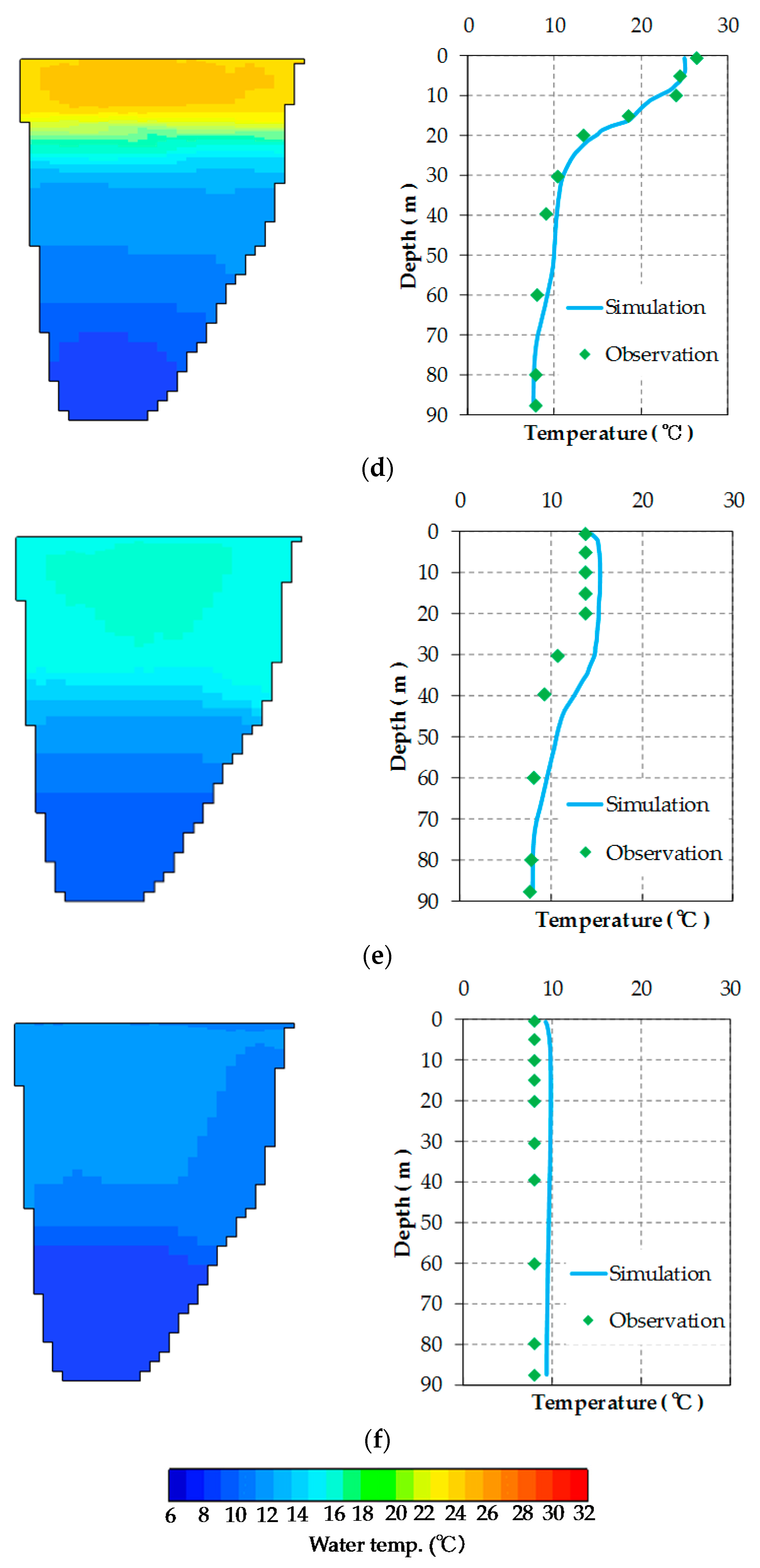
The water distributions along the line passing from west to east through the monitoring point in Imazu-oki are shown in Figure 6. The snapshots were taken at 12:00 p.m. from April 2007 to February 2008 every two months. The vertical distributions of water temperature each year are not very different from each other; accordingly, we picked the values in 2007 as a representative year for the current analysis. As is evident in the observations, the water temperature of the surface rises from spring to summer, and the stratification becomes strong. However, the mixed layer is formed by the mixing of the wind in the surface layer. The difference between the surface layer and the bottom layer becomes large, and the thermocline is formed as a result. The thickness of the thermocline increases as the air temperature rises.
In a stratified season, the water temperature on the eastern coast rises slightly higher than that of the central and western coasts. As the water depth on the eastern coast is shallower than the ones on the central and western coasts, the water parcel on the eastern coast is heated more easily than in other places. Therefore, the stratification tilts slightly. In the cooling season, the surface of the lake cools down as the air temperature decreases. Due to the cooling flux and the effect of the wind, the thermocline deepens. In addition, since the water depth on the eastern coast is shallower than the one on the central and western coasts, the water parcel on the eastern coast is cooled more easily than in other places, as shown in Figure 6d–f. The stratification again tilts slightly due to the nonuniformity in the topography of the bottom. In December, there is still little difference in the water temperature between the surface and the bottom of the lake. In February, the water temperature of all layers cools down and becomes uniform. The stratification distinguishes in the middle of winter.
3.2.2. Inter-Annual Change of the Vertical Distribution of Water Temperature at the Monitoring Point in Imazu-Oki
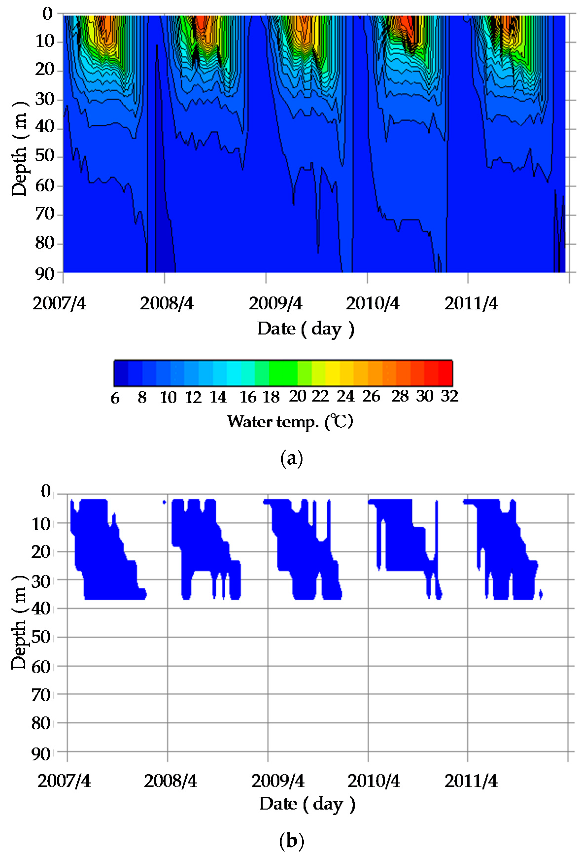
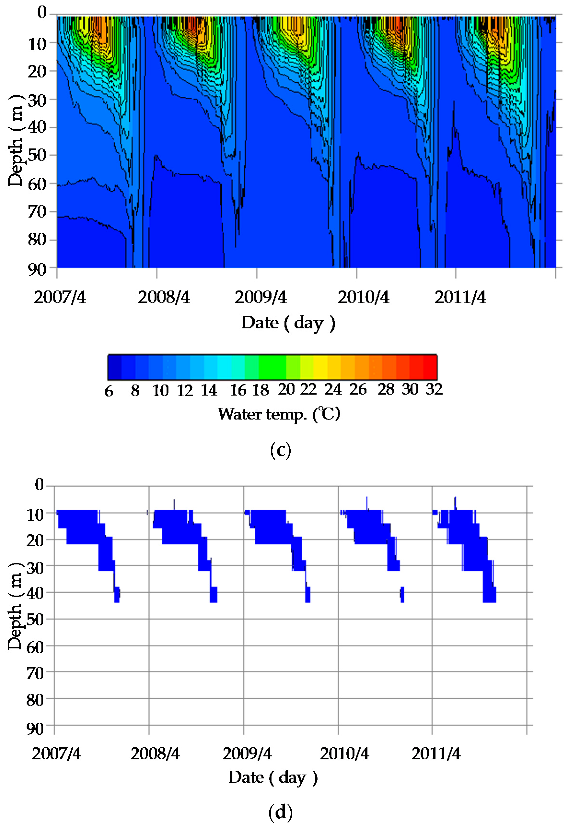
Inter-annual change in the vertical profiles of observed and simulated water temperatures at the monitoring point in Imazu-oki are represented in Figure 7. As shown in Figure 7a, the water temperature is projected by using the ten observed data intervals. In summer, the temperature of the surface water rises to about 27 °C; however, the temperature of the bottom water is about 7 °C. Because of this vertical difference of water temperature, a thermocline is formed. The observed water temperature is higher than the simulated value, so stratification is slightly stronger. Additionally, as shown in Figure 7a,c, the climate in winter and early spring of 2007 (where the average air temperature in January–March was 9.4 °C) was warmer than in other years (where the average air temperature in January–March was 7.8 °C). This led to the strong stratification in 2007.
On the other hand, since weather in the summer of 2009 (where the average air temperature in July–September was 23.9 °C) was cooler than in other years (where the average air temperature in July–September was 25.2 °C), the stratification was weaker than in other years. In winter, the water temperature of all layers became uniform due to the vertical mixing in the simulation.
We investigated the thickness of the thermocline in the study region. The thermocline is defined as the area where the change of the water temperature is more than 0.1 °C/m in the vertical direction. After calculating the gradient of water temperature from the surface layer to the bottom layer, the area where the gradient is over 0.1 °C/m are shown in Figure 7b,d. As shown in Figure 7b,d, the observed trend of the thickness of the thermocline is well reproduced by the simulation. In summer, the thickness of the simulation is thinner than observations. From autumn, the thermocline begins to disappear, and in winter the water parcel is mixed well.
3.2.3. Flow Field in the Lake
For the validation of the model, we confirmed the presence of circulation in the lake. In addition, the currents of circulation flow play an important role in the transportation and mixing of dissolved or suspended materials. The significant feature of the flow field in Lake Biwa is the system of several circulations formed in the surface layer of the southern part of the lake. In the 1920s, there were considered to be three main circulation flows: the first circulation flow (anticlockwise), the second circulation flow (clockwise), and the third circulation flow (anticlockwise). However, since the 1980s, the development of flow velocity measuring equipment with mooring or with the bottom of a ship made it possible to clarify the features of the flow field in detail. It was pointed out that the third circulation flow did not exist; therefore, there were only two circulation flows [40]. These surface circulations have also been observed in other large lakes [41]. In Lake Superior, Lake Erie, Lake Constance, etc., anticlockwise circulations have been observed. Basin shape and depth distribution, as well as the size of the lake affect the circulations.
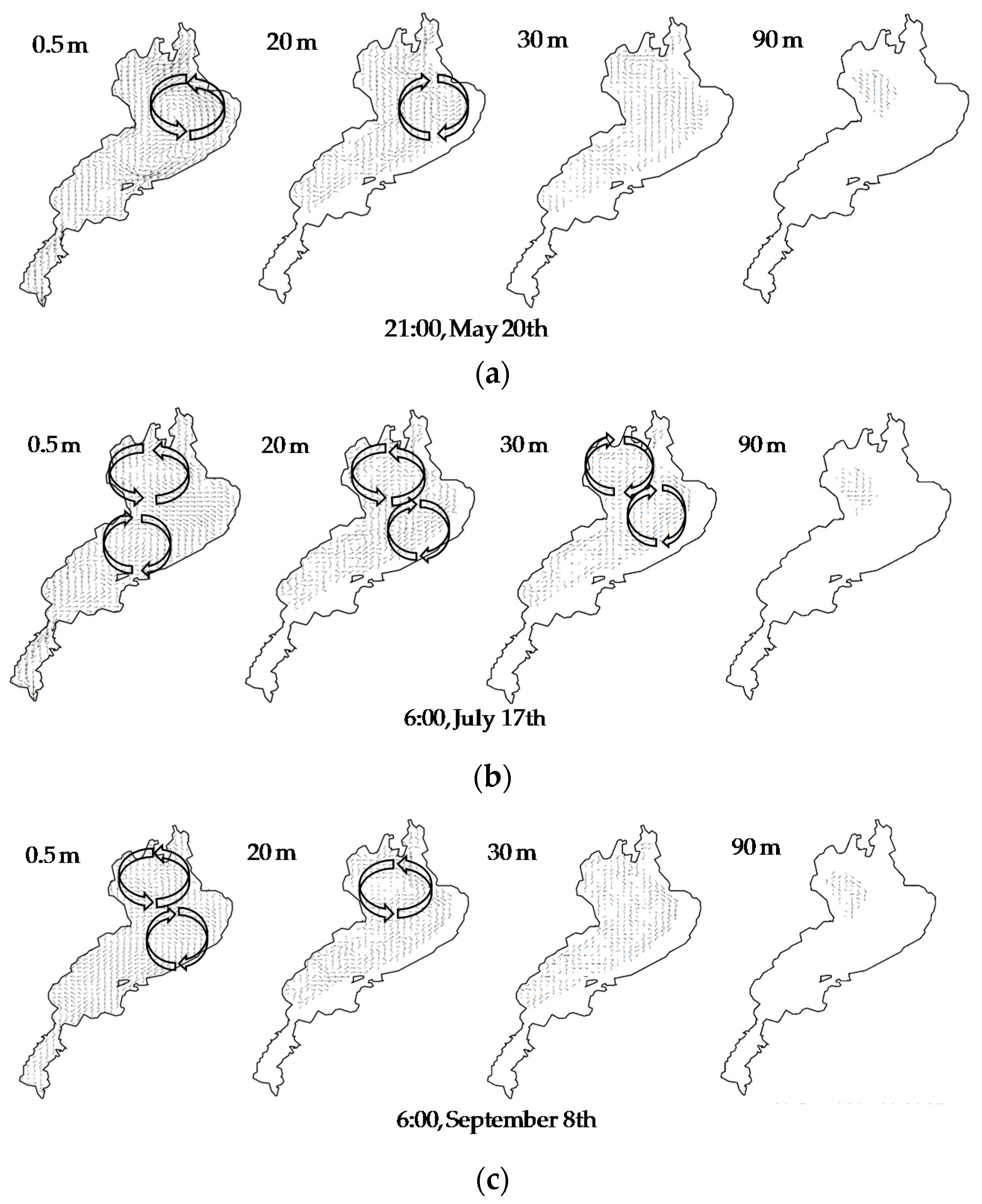
In this study, the results were collected every three hours and were drawn in a horizontal cross-sectional view of the surface layer. The snapshot results of the flow field in each layer are shown in Figure 8a–e. The first circulation flow appears above the thermocline and continues to show up from May to November (Figure 8a–d). The velocity is about 10–30 cm/s, peaking in the summer. In the bottom layer, there is a subtle flow each month (Figure 8a–e). As shown in Figure 8a, the first circulation flow exists in the center of the circle in the northern part of the lake. In order to compensate for the flow field in the surface layer, the clockwise circulation exists right under the thermocline. There is a subtle circulation flow in the bottom layer. Figure 8b represents the results on 17 July. We confirmed the presence of the first circulation flow (anticlockwise) in the northern part of the lake and the second circulation flow (clockwise) in the southern part of the lake from the surface layer to the thermocline. As is the case with results on 20 May, the clockwise circulation exists right under the thermocline (Figure 8b). There is also a subtle flow in the bottom layer.
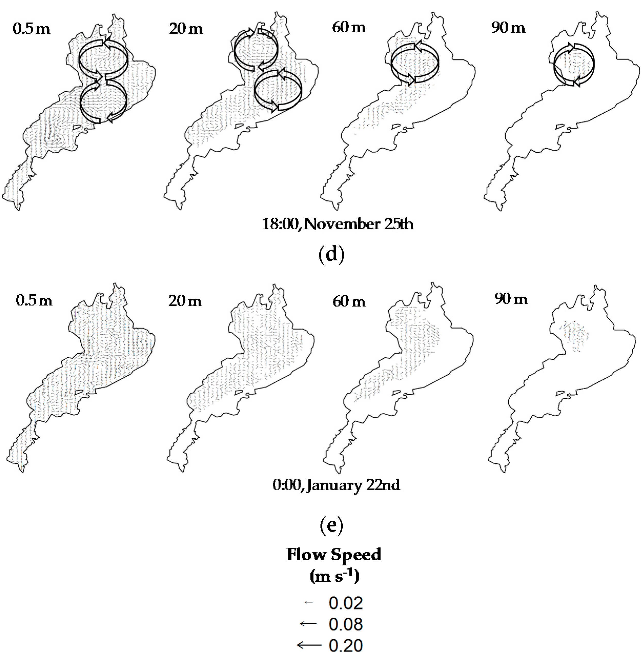
In autumn, as air temperature cools down, the thermocline begins to fall. In addition, typhoons control the flow dynamics in the autumn season. As a result, the wind affects the surface flow more directly and it becomes difficult to constantly form the circulation flow in the surface layer. However, the anticlockwise circulation flow is formed in the surface layer and the thermocline in the northern part of the lake according to Figure 8c (on 8 September). Under the thermocline, there is a clockwise circulation flow different from the layers above. In November, the thermocline starts to disappear. From the surface layer to the deep layer (Figure 8d), the anticlockwise circulation flow still exists and the clockwise circulation flow is formed in the north part of the anticlockwise circulation in the deep layer. During the middle of winter, there are some circulation flows in the surface layer; however, the strong circulation flow could not be confirmed consistently. In the deep layer, there are some circulation flows which were not shown in the figures. For the majority of the days, there was no strong circulation flow, as shown in Figure 8e.
4. Conclusions
In the present study, we built a three-dimensional hydrodynamic model and evaluated the reproducibility of the structure of the thermal stratification and flow field in Lake Biwa. Numerical simulation was carried out for a time period from 2007 to 2011. As a result, we reproduced the structure of the stratification as observed.
Although simulated water temperature of the surface layer is a little lower than the observed value, the vertical distribution of water temperature in the simulation agrees with observations based on the statistical analysis. The model was able to reproduce the seasonal variation of the structure of the stratification and vertical mixing in winter. In spring, the stratification begins and becomes strong during summer. The difference of the strength of the stratification depends on the mean air temperature during the stratified season each year. In autumn, the stratification starts to diminish and the overturning occurs in the middle of winter.
In the present model, the vertical water distribution during autumn and winter cannot be reproduced well. This is because the cooling flux is not transferred to the deep layer. The model should be improved by using a certain model which accounts for the effect of the wind to the deep layer precisely.
It is important to grasp the inter-annual and seasonal changes of the structure of the stratification in order to evaluate whether or not dissolved oxygen—which affects the aquatic life—is supplied to the deep layers in the future. Due to the fact that stratification is affected—depending on the water depth—by (1) the difference of the water temperature in the horizontal direction and (2) the difference of volume for advection-diffusion due to the amount of heat, it is necessary to reproduce the flow field in all layers for precise prediction of stratification.
The circulation flow in the surface layer was reproduced well. The first anticlockwise circulation flow exists in the center of the circle in the northern part of the lake during stratified seasons, similar to the observations. In addition, in order to compensate for the flow field in the surface layer, the clockwise circulation exists right under the thermocline. The present model experiments reproduced the structure of the stratification and the flow field in Lake Biwa based on observations. The overall results will help to understand the movement of the substances in all layers of the lake.
Acknowledgments
The meteorological data in Shiga Prefecture were provided by Japan Meteorological Agency, and water-quality data were given by Lake Biwa Environmental Research Institute via Internet. The authors are grateful for these support.
Author Contributions
Jinichi Koue designed and performed the experiments, analyzed the data and wrote the paper; Hikari Shimadera, Tomohito Matsuo, and Akira Kondo contributed to building the model, preparing the input data and providing important suggestions on the data analysis. All the authors have read and approved the final manuscript.
Conflicts of Interest
The authors declare no conflict of interest.
References
- Livingstone, D.M. Impact of secular climate change on the thermal structure of a large temperate central European lake. Clim. Chang. 2003, 57, 205–225. [Google Scholar] [CrossRef]
- Intergovernmental Panel on Climate Change. The physical science basis. In Contribution of Working Group I to the Fifth Assessment Report of the Intergovernmental Panel on Climate Change; Cambridge University Press: Cambridge, UK, 2013. [Google Scholar]
- Straile, D.; Jöhnk, K.; Rossknecht, H. Complex effects of winter warming on the physicochemical characteristics of a deep lake. Limnol. Oceanogr. 2003, 48, 1432–1438. [Google Scholar] [CrossRef]
- Brooks, A.S.; Zastrow, J.C. The potential influence of climate change on offshore primary production in Lake Michigan. Great Lakes Res. 2002, 28, 597–607. [Google Scholar] [CrossRef]
- Livingstone, D.M. A change of climate provokes a change of paradigm: Taking leave of two tacit assumptions about physical lake forcing. Int. Rev. Hydrobiol. 2008, 93, 404–414. [Google Scholar] [CrossRef]
- Coats, R.; Perez-Losada, J.; Schladow, G.; Richards, R.; Goldman, C. The warming of Lake Tahoe. Clim. Chang. 2006, 76, 121–148. [Google Scholar] [CrossRef]
- Danis, P.A.; Von Grafenstein, U.; Masson-Delmotte, V.; Planton, S.; Gerdeaux, D.; Moisselin, J.M. Vulnerability of two European lakes in response to future climate changes. Geophys. Res. Lett. 2004, 31, L21507. [Google Scholar] [CrossRef]
- Matzinger, A.; Schmid, M.; Veljanoska-Sarafiloska, E.; Patceva, S.; Guseska, D.; Wagner, B.; Müller, B.; Sturm, M.; Wüest, A. Eutrophication of ancient Lake Ohrid: Global warming amplifies detrimental effects of increased nutrient inputs. Limnol. Oceanogr. 2007, 52, 338–353. [Google Scholar] [CrossRef]
- Endoh, S.; Yamashita, S.; Kawakami, M.; Okumura, Y. Recent warming of Lake Biwa water. Jpn. J. Limnol. 1999, 60, 223–228. (In Japanese) [Google Scholar] [CrossRef]
- Peeters, F.; Livingstone, D.M.; Goudsmit, G.-H.; Kipfer, R.; Forster, R. Modeling 50 years of historical temperature profiles in a large central European lake. Limnol. Oceanogr. 2002, 47, 186–197. [Google Scholar] [CrossRef]
- Arhonditsis, G.B.; Brett, M.T.; DeGasperi, C.L.; Schindler, D.E. Effects of climatic variability on the thermal properties of Lake Washington. Limnol. Oceanogr. 2004, 49, 256–270. [Google Scholar] [CrossRef]
- Yoshimizu, T.; Yoshiyama, K.; Tayasu, I.; Koitabashi, T.; Nagata, T. Vulnerability of a large monomictic lake (Lake Biwa) to warm winter event. Limnology 2010, 11, 233–239. [Google Scholar] [CrossRef]
- Stocker, R.; Imberger, J. Horizontal transport and dispersion in the surface layer of a medium-sized lake. Limnol. Oceanogr. 2003, 48, 971–982. [Google Scholar] [CrossRef]
- Saggio, A.; Imberger, J. Internal wave weather in a stratified lake. Limnol. Oceanogr. 1998, 43, 1780–1795. [Google Scholar] [CrossRef]
- Shimizu, K.; Imberger, J.; Kumagai, M. Horizontal structure and excitation of primary motions in a strongly stratified lake. Limnol. Oceanogr. 2007, 52, 2641–2655. [Google Scholar] [CrossRef]
- Shimizu, K.; Imberger, J. Energetics and damping of basin-scale internal waves in a strongly stratified lake. Limnol. Oceanogr. 2008, 53, 1574–1588. [Google Scholar] [CrossRef]
- Kitazawa, D.; Ishikawa, T.; Kumagai, M. The analysis by the numerical simulation about the effects of the climate change for the past 50 years on an ecological system. Inst. Ind. Sci. 2010, 62, 45–49. (In Japanese) [Google Scholar]
- Kitazawa, D.; Kumagai, M.; Hasegawa, N. Effects of Internal Waves on Dynamics of Hypoxic Waters in Lake Biwa. J. Korean Soc. Mar. Environ. Eng. 2010, 13, 30–42. [Google Scholar]
- Fer, I.; Lemmin, U.; Thorpe, S.A. Observations of mixing near the sides of a deep lake in winter. Limnol. Oceanogr. 2002, 47, 535–544. [Google Scholar] [CrossRef]
- Akitomo, K.; Tanaka, K.; Kumagai, M.; Jiao, C. Annual cycle of circulations in Lake Biwa, part 1: Model validation. Limnology 2009, 10, 105–118. [Google Scholar] [CrossRef]
- Akitomo, K.; Tanaka, K.; Kumagai, M. Annual cycle of circulations in Lake Biwa, part 2: Mechanisms. Limnology 2009, 10, 119–129. [Google Scholar] [CrossRef]
- Kumagai, M.; Vincent, W.F.; Ishikawa, K.; Aota, Y. Lessons from Lake Biwa and Other Asian Lakes: Global and Local Perspectives, Freshwater Management, Global Versus Local Perspectives; Springer: Tokyo, Japan, 2003; Chapter 1; pp. 1–22. [Google Scholar]
- Akitomo, K.; Kurogi, M.; Kumagai, M. Numerical study of a thermally induced gyre system in Lake Biwa. Limnology 2004, 5, 103–114. [Google Scholar] [CrossRef]
- Kitazawa, D.; Kumagai, M. Numerical simulation on seasonal variation in dissolved oxygen tension in Lake Biwa. In Proceedings of the 2nd Joint Japan/Korea Workshop on Marine Environmental Engineering, Kasuga, Japan, 21–22 October 2005; pp. 71–90. [Google Scholar]
- Gholami, V.; Chau, K.W.; Fadaee, F.; Tarkaman, J.; Ghaffari, A. Modeling of groundwater level fluctuations using dendrochronology in alluvial aquifers. J. Hydrol. 2015, 529, 1060–1069. [Google Scholar] [CrossRef]
- Taormina, R.; Chau, K.W.; Sivakumar, B. Neural network river forecasting through baseflow separation and binary-coded swarm optimization. J. Hydrol. 2015, 529, 1788–1797. [Google Scholar] [CrossRef]
- Wu, C.L.; Chau, K.W.; Fan, C. Prediction of rainfall time series using modular artificial neural networks coupled with data-preprocessing techniques. J. Hydrol. 2010, 389, 146–167. [Google Scholar] [CrossRef]
- Kantha, L.H.; Clayson, C.A. An improved mixed layer model for geophysical applications. J. Geophys. Res. 1994, 99, 25235–25266. [Google Scholar] [CrossRef]
- Goudsmit, G.H.; Burchard, H.; Peeters, F.; Wüest, A. Application of k-ϵ turbulence models to enclosed basins: The role of internal seiches. J. Geophys. Res. Oceans 2002, 107, 3230–3242. [Google Scholar] [CrossRef]
- MacIntyre, S.; Clark, J.F.; Jellison, R.; Fram, J.P. Turbulent mixing induced by nonlinear internal waves in Mono Lake, California. Limnol. Oceanogr. 2009, 54, 2255–2272. [Google Scholar] [CrossRef]
- Ishizuka, H.; Kitazawa, D.; Konno, A. A Feasibility Study of Turbulence Models for Numerical Simulation of Physical Environment in Lake Biwa. In Proceedings of the 19th Symposium in Computational Fluid Dynamics, Tokyo, Japan, 13–15 December 2005; pp. 1–10. (In Japanese). [Google Scholar]
- Mellor, G.L.; Yamada, T. Development of a turbulence closure model for geophysical fluid problems. Rev. Geophys. Space Phys. 1982, 20, 851–875. [Google Scholar] [CrossRef]
- Burchard, H.; Baumert, H. On the performance of a mixed-layer model based on the κ–ϵ turbulence closure. J. Geophys. Res. 1995, 100, 8523–8540. [Google Scholar] [CrossRef]
- Munk, W.H.; Anderson, E.R. Notes on a theory of the thermocline. J. Mar. Res. 1948, 7, 276–295. [Google Scholar]
- Webb, E.K. Profile relationships: The log-linear range, and extension to strong stability. Q. J. R. Meteorol. Soc. 1970, 96, 67–90. [Google Scholar] [CrossRef]
- Kondo, J. Fundamentals of the surface heat balance. In Meteorology of Water Environment; Asakura Publishing: Tokyo, Japan, 1994; Chapter 6; pp. 132–159. (In Japanese) [Google Scholar]
- Kondo, J. Air-sea bulk transfer coefficients in diabatic conditions. Bound. Layer Meteorol. 1975, 9, 91–112. [Google Scholar] [CrossRef]
- Hirose, N.; Kim, C.H.; Yoon, J.H. Heat budget in the Japan Sea. J. Oceanogr. 1996, 52, 553–574. [Google Scholar] [CrossRef]
- Shrestha, K.L.; Kondo, A. Assessment of the Water Resource of the Yodo River Basin in Japan Using a Distributed Hydrological Model Coupled with WRF Model. In Environmental Management of River Basin Ecosystems; Part of the Series Springer Earth System Sciences; Springer: Berlin, Germany, 2015; pp. 137–160. [Google Scholar]
- Endoh, S.; Okumura, Y. Gyre system in Lake Biwa derived from recent current measurements. Limnology 1993, 54, 191–197. [Google Scholar] [CrossRef]
- Emercy, K.O.; Csanady, G.T. Surface circulation of lakes and nearly land-locked seas. Proc. Natl. Acad. Sci. USA 1973, 70, 93–97. [Google Scholar] [CrossRef]
Figure 1.
(a) The location of Lake Biwa in Japan; (b) the location of rivers; (c) the water depth of Lake Biwa.
Figure 1.
(a) The location of Lake Biwa in Japan; (b) the location of rivers; (c) the water depth of Lake Biwa.


Figure 2.
Time series of (a) Air temperature; (b) Wind speed; and (c) Short-wave radiation for boundary conditions from 2007 to 2012.
Figure 2.
Time series of (a) Air temperature; (b) Wind speed; and (c) Short-wave radiation for boundary conditions from 2007 to 2012.

Figure 3.
Vertical distribution of the mean value and standard deviation of the water temperature from 2007 to 2011 at the monitoring point in Imazu-oki in (a) April to June; (b) July to September; (c) October to December; and (d) January to March.
Figure 3.
Vertical distribution of the mean value and standard deviation of the water temperature from 2007 to 2011 at the monitoring point in Imazu-oki in (a) April to June; (b) July to September; (c) October to December; and (d) January to March.

Figure 4.
Time series of short-wave radiation, net long-wave radiation, latent heat flux, and sensible heat flux from 2007 to 2012.
Figure 4.
Time series of short-wave radiation, net long-wave radiation, latent heat flux, and sensible heat flux from 2007 to 2012.

Figure 5.
Time series of observed and simulated water temperature at depths of 0.5 m, 20 m, and 90 m at the monitoring point in Imazu-oki.
Figure 5.
Time series of observed and simulated water temperature at depths of 0.5 m, 20 m, and 90 m at the monitoring point in Imazu-oki.

Figure 6.
Seasonal change in vertical distribution of simulated water temperature (Color contour: Temperature (°C)) (a) 3 April; (b) 4 June; (c) 6 August; (d) 1 October; (e) 3 December; and (f) 4 February.
Figure 6.
Seasonal change in vertical distribution of simulated water temperature (Color contour: Temperature (°C)) (a) 3 April; (b) 4 June; (c) 6 August; (d) 1 October; (e) 3 December; and (f) 4 February.


Figure 7.
Inter-annual change of (a) the vertical water distribution and (b) the thickness of the thermocline at the monitoring point in Imazu-oki in the observation; and (c) the vertical water distribution and (d) the thickness of the thermocline at the same point in the simulation.
Figure 7.
Inter-annual change of (a) the vertical water distribution and (b) the thickness of the thermocline at the monitoring point in Imazu-oki in the observation; and (c) the vertical water distribution and (d) the thickness of the thermocline at the same point in the simulation.


Figure 8.
Flow field in each layer from May of 2007 to January of 2008 (a) 20 May; (b) 17 July; (c) 8 September; (d) 25 November; (e) 22 January.
Figure 8.
Flow field in each layer from May of 2007 to January of 2008 (a) 20 May; (b) 17 July; (c) 8 September; (d) 25 November; (e) 22 January.


Table 1.
Statistical indicators between the observed and simulated data (mean values for 5 years). MAE: mean absolute error; MB: mean bias.
Table 1.
Statistical indicators between the observed and simulated data (mean values for 5 years). MAE: mean absolute error; MB: mean bias.
| All Layers | Seasonal Index | Annual Index | |||
| Spring | Summer | Autumn | Winter | ||
| r | 0.95 | 0.98 | 0.96 | 0.88 | 0.97 |
| MAE (°C) | 0.9 | 1.1 | 1.2 | 1.3 | 1.1 |
| MB (°C) | 0.5 | 0.0 | 1.1 | 1.3 | 0.7 |
| 0.5 m | Seasonal Index | Annual Index | |||
| Spring | Summer | Autumn | Winter | ||
| r | 0.97 | 0.92 | 0.99 | 0.91 | 0.99 |
| MAE (°C) | 1.1 | 1.7 | 0.6 | 0.9 | 1.1 |
| MB (°C) | 0.6 | −1.7 | 0.1 | 0.9 | 0.0 |
| 20 m | Seasonal Index | Annual Index | |||
| Spring | Summer | Autumn | Winter | ||
| r | 0.81 | 0.62 | 0.61 | 0.62 | 0.87 |
| MAE (°C) | 0.8 | 1.5 | 1.9 | 1.4 | 1.4 |
| MB (°C) | −0.3 | 0.6 | 1.9 | 1.4 | 0.9 |
| 90 m | Seasonal Index | Annual Index | |||
| Spring | Summer | Autumn | Winter | ||
| r | −0.04 | 0.06 | 0.20 | 0.70 | 0.27 |
| MAE (°C) | 0.6 | 0.4 | 0.5 | 1.1 | 0.7 |
| MB (°C) | 0.4 | 0.3 | 0.5 | 1.1 | 0.6 |
© 2018 by the authors. Licensee MDPI, Basel, Switzerland. This article is an open access article distributed under the terms and conditions of the Creative Commons Attribution (CC BY) license (http://creativecommons.org/licenses/by/4.0/).
Share and Cite
MDPI and ACS Style
Koue, J.; Shimadera, H.; Matsuo, T.; Kondo, A. Evaluation of Thermal Stratification and Flow Field Reproduced by a Three-Dimensional Hydrodynamic Model in Lake Biwa, Japan. Water 2018, 10, 47. https://doi.org/10.3390/w10010047
AMA Style
Koue J, Shimadera H, Matsuo T, Kondo A. Evaluation of Thermal Stratification and Flow Field Reproduced by a Three-Dimensional Hydrodynamic Model in Lake Biwa, Japan. Water. 2018; 10(1):47. https://doi.org/10.3390/w10010047
Chicago/Turabian StyleKoue, Jinichi, Hikari Shimadera, Tomohito Matsuo, and Akira Kondo. 2018. "Evaluation of Thermal Stratification and Flow Field Reproduced by a Three-Dimensional Hydrodynamic Model in Lake Biwa, Japan" Water 10, no. 1: 47. https://doi.org/10.3390/w10010047
Note that from the first issue of 2016, this journal uses article numbers instead of page numbers. See further details here.