Studying Operation Rules of Cascade Reservoirs Based on Multi-Dimensional Dynamics Programming

School of Hydropower & Information Engineering, Huazhong University of Science and Technology, Wuhan 430074, China
*
Author to whom correspondence should be addressed.
Water 2018, 10(1), 20; https://doi.org/10.3390/w10010020
Submission received: 29 October 2017
/
Revised: 19 December 2017
/
Accepted: 25 December 2017
/
Published: 27 December 2017
(This article belongs to the Special Issue Planning and Operations of Multi-Objective River and Reservoir Systems)
Abstract
:Although many optimization models and methods are applied to the optimization of reservoir operation at present, the optimal operation decision that is made through these models and methods is just a retrospective review. Due to the limitation of hydrological prediction accuracy, it is practical and feasible to obtain the suboptimal or satisfactory solution by the established operation rules in the actual reservoir operation, especially for the mid- and long-term operation. In order to obtain the optimized sample data with global optimality; and make the extracted operation rules more reasonable and reliable, this paper presents the multi-dimensional dynamic programming model of the optimal joint operation of cascade reservoirs and provides the corresponding recursive equation and the specific solving steps. Taking Li Xianjiang cascade reservoirs as a case study, seven uncertain problems in the whole operation period of the cascade reservoirs are summarized after a detailed analysis to the obtained optimal sample data, and two sub-models are put forward to solve these uncertain problems. Finally, by dividing the whole operation period into four characteristic sections, this paper extracts the operation rules of each reservoir for each section respectively. When compared the simulation results of the extracted operation rules with the conventional joint operation method; the result indicates that the power generation of the obtained rules has a certain degree of improvement both in inspection years and typical years (i.e., wet year; normal year and dry year). So, the rationality and effectiveness of the extracted operation rules are verified by the comparative analysis.
1. Introduction
Hydropower is one of the cleanest energy sources that can be commercially developed on a large scale [1]. It has exceptional advantages when compared with other energy sources [2,3], such as pollution-free, renewable, manageable, and so on. Moreover, hydropower has the unique ability to change the output quite fast, which makes it good at meeting the changing demands for electricity. These advantages of hydropower have drawn the attention of the optimization research of reservoir operation all over the world [4,5].
The optimal operation of reservoirs is spatial and temporal redistribution of water resources to bring benefit and eliminate harm by using the hydraulic connection, power connection, and storage compensation between the upstream and downstream reservoirs. At present, with the completion of large cascade reservoirs system, how to manage and which rules to follow to play the biggest benefit of cascade reservoirs have become the urgent issues [6,7]. The deterministic optimization results often contain a large amount of regular information, and this information has great significance in guiding the actual operation of cascade reservoirs [8,9]. Therefore, it is one of the most effective ways to solve the above issues by mining the regularity of operation and extracting the appropriate operation rules based on the optimization results [10]. The optimization results can be obtained by solving the operation optimization model of cascade reservoirs, according to appropriate optimization algorithms and the long series of historical runoff data [11,12]. The extracted operation rules can be then used to guide the actual operation of cascade reservoirs. On the whole, a good optimized operation rule can improve the power generation of hydropower stations by about 1~3% compared with the traditional operation methods [13,14].
Nowadays, there are mainly two kinds of optimization algorithms that are used to solve the operation optimization model of cascade reservoirs. One kind is the traditional and classical optimization methods, such as dynamic programming (DP) and its improved methods [15,16]. The other kind is the intelligent optimization algorithms [17]. DP is a multi-stage optimization algorithm and it has a global convergence. Nowadays, DP is widely used in the optimization of single reservoir operation. The most significant characteristic of DP is able to obtain the global optimal solution, and it has no requirement for the initial trajectory. But, the emergence of “curse of dimensionality” limited its application in the operation optimization of large cascade reservoirs [18]. Accordingly, the improved DP algorithms are often adopted in the optimization to avoid the “curse of dimensionality”, such as discrete differential dynamic programming [19], dynamic programming with successive approximation [20], progressive optimality algorithm [21], incremental dynamic programming [22], and stochastic dual dynamic programming [23], etc. However, due to the convergence of the algorithms themselves, although these improved algorithms can effectively avoid the “curse of dimensionality” to some extent in the operation optimization of large cascade reservoirs, only the approximate theoretical optimal solution of the problem can be obtained in most cases.
For the intelligent optimization algorithms, such as particle swarm optimization [24], genetic algorithm [25], differential evolution algorithm [26], ant colony optimization [27], and so on, because they can be directly applied to deal with the complex problems with characteristics of nonlinear, discontinuous, non-differentiable, and multi-dimensional, they are widely used in the optimization of cascade reservoirs. Plenty of intelligent optimization algorithms have been proved to possess a global convergence, but they cannot guarantee a global optimum with finite iterations that are affected by the stochastic feature. Meanwhile, their solutions are limited by the calculation time and constraints in some certain optimization [28].
Reservoir operation rules are usually extracted based on the regular information of sample data [29]. So, the optimal nature of sample data will directly determine the rationality and validity of the extracted operation rules. However, the optimal nature of the sample data depends on the performance of the algorithm that is used in solving the model. Thus, whether the optimization algorithm has a global convergence or not determines the rationality and validity of the extracted operation rules. In order to obtain the sample data with global optimality, and extract the optimal operation rules consistent with the actual situation, this paper proposed the Multi-dimensional Dynamic Programming (MDP) model to solve the operation optimization of cascade reservoirs. Therefore, the global optimality of the calculation results (sample data) can be guaranteed by the global convergence of MDP. A detailed case study was presented in this paper by taking the Li Xianjiang cascade reservoirs in China as an instance. After the analysis and summarization for the optimal sample data, this paper proposed seven uncertain problems in the whole operation period of the cascade reservoirs, and put forward two sub-models to solve these uncertain problems. At last, this paper extracted the operation rules for each reservoir by taking the water level as the decision variable and dividing the whole operation period of each reservoir into four characteristic sections. The simulation results between the extracted rules and the conventional method were compared and analyzed in detail to evaluate the performance of the extracted operation rules.
2. Operation Optimization Model of Cascade Reservoirs
2.1. Objective Function
The optimization of cascade reservoirs aims at maximizing the power generation by developing an optimal plan over the entire planning horizon [30,31], while satisfying all kinds of physical and operational constraints. Generally, its objective function can be expressed as follows.
where E is the total power generation over the entire planning horizon, unit: kWh; T is the number of stages over the entire planning horizon; is the output of the ith hydropower station in the tth stage, unit: kW, and the reservoir indexes are 1, 2, ... , n from upstream to downstream in this paper; Δt is the duration of a stage, unit: h; TN is the total guaranteed output of cascade hydropower stations; A is the penalty coefficient, and it is used for the situation when the actual total output of cascade hydropower stations is lower than TN; σt is a 0–1 variable, and its value can be expressed as follows [32]:
2.2. Main Constraints
- (1)
- Water balance constraints
- (2)
- Reservoir volume limits
- (3)
- Comprehensive utilization limits of water resources required at downstream
- (4)
- Output limits
- (5)
- Boundary conditions limits
3. Multi-Dimensional Dynamic Programming
3.1. Basic Principle
Reservoir operation optimization can be regarded as a multi-stage decision problem, and the whole operation period can be divided into T discretized stages when we use the DP to solve it. A month represents a stage in this paper. The storage volume of reservoir at the end of each stage is the volume at the beginning of the next stage, this means the storage volume at the beginning of each stage is only related to the storage volume at the end of the previous stage, and it has nothing to with the other stages. So, the operation optimization of reservoir by DP satisfies the principle of “unfollow-up effect”. In addition, the water balance Equation (3) reflects the conversion relationship of storage volume between the adjacent two stages. Therefore, the recursive equation of the deterministic DP model in the operation optimization of single reservoir can be described as follows [34]:
where Vt is the state variable; Qt is the decision variable, and it is determined by beginning state , and end state ; m1 is state index at the beginning of a stage, and m1 = 1, 2, …, M; m2 is the state index at the end of a stage, and m2 = 1, 2, …, M; M is the number of discrete points of storage volume; Dt is the decision variables set in the tth stage; Nt() is the output function in the tth stage; is the optimal cumulative output of state m1 at the beginning of tth stage, unit: kW; is the optimal cumulative output of the state m2 at the beginning of (t + 1)th stage, unit: kW. The optimal cumulative output means the sum of the output in the optimal output process from present stage t to last stage T. The output is calculated up to the first stage in the reverse recursion procedure, which starts from the last stage, and the water level route of the optimal operation can be obtained at last by the calculation with a chronological order recursion procedure.
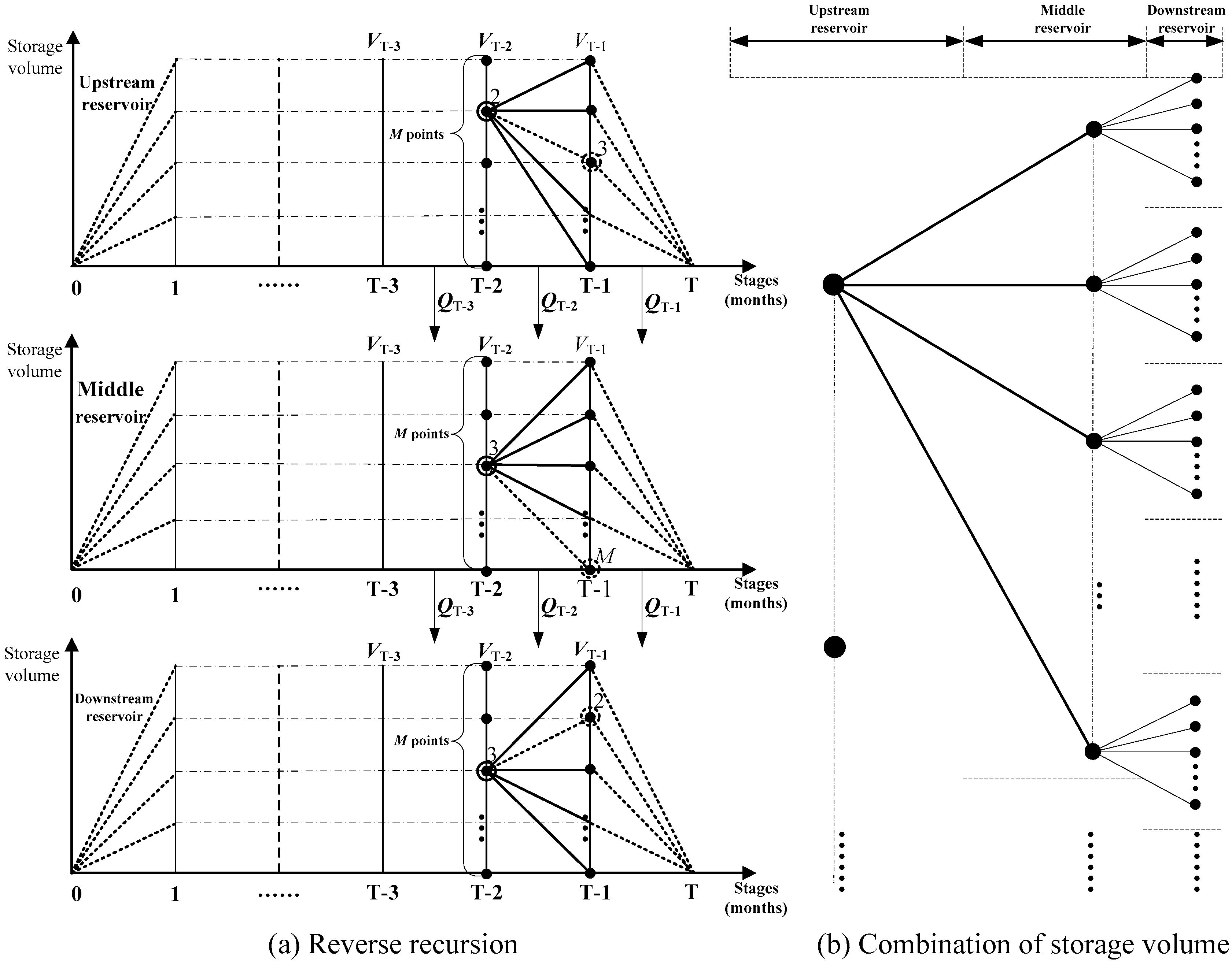
However, because the number of reservoirs is often two or more in a cascade reservoirs system [35], many variables and constraints are integrated in the procedure of solving the operation optimization of cascade reservoirs. If the number of discrete points of storage volume for each reservoir is M in a cascade system consisting of three reservoirs, then M3 combinations of these discrete points can be obtained in each stage. Referring to the reverse recursion procedure of DP in the operation optimization of single reservoir, we can get the optimal combination of storage volume for each stage by taking each combination as a state and implementing the reverse recursion. The combination principle of discretized storage volume is shown in Figure 1b, and the recursive equation of MDP can be formulated as follows:
where Qt = (, , …, )′ is the decision variable vector; Vt−1 = (, , …, )′ is the state variable vector. In formula (10), because of the discretization, is equivalent to (, , …, ), is equivalent to (, ,…, ), and is equivalent to (, , …, ); is the optimal cumulative output of a combination of storage volume at the tth stage, unit: kW; is the optimal cumulative output of a combination of storage volume at the (t + 1)th stage, unit: kW.
3.2. Calculation Procedure of MDP
The reverse recursion procedure of MDP in the optimization of cascade reservoirs can be described as follows.
Step 1: In the last stage T, there are M discretized points for the storage volume of each reservoir at the beginning of this stage, and M3 combinations of these discretized points can be obtained, and each combination contains three discretized points. Because the storage volumes are fixed at the end of this stage, the optimal candidate path of each combination is unique at this moment.
Step 2: In stage T − 1, the storage volumes of each reservoir are not fixed at the end of this stage, so there are also M discretized points for the storage volume of each reservoir and M3 combinations for these discretized points. For any combination at the beginning of this stage, such as combination (2, 3, 3), which, respectively, represents a discretized point for upstream, midstream, and downstream reservoir, as shown in Figure 1a, with the solid line circle, we can find out the optimal candidate path that corresponds to combination (2, 3, 3) by traversing all M3 combinations of the storage volume at the end of this stage. Assuming that it is the combination (3, M, 2), as shown in Figure 1a with the dotted line circle, and then save the optimal candidate path and the cumulative output of combination (2, 3, 3) in the memory for the usage of next stage.
Step 3: Repeats step 2, then the calculation of stage T − 1 can be finished by implementing the same work for the other M3-1 combinations of the storage volume at the beginning of this stage, except for combination (2, 3, 3).
Step 4: Repeat steps 2 and 3, then the whole calculation of all stages over the entire planning horizon can be finished by this reverse recursion procedure, and the optimal candidate path of each combination and its optimal cumulative output can be obtained after the calculation.
Step 5: Similar to DP in solving the operation optimization of single reservoir, the route, and other details of the optimal operation can ultimately be obtained in chronological recursion process.
Nowadays, many achievements about the application of DP in the reservoir operation and management are available for reference, and they can be found in the literature by Nandalal et al. [37]. Here is an application of MDP to the operation rule extraction of multi-reservoirs in this paper.
4. Case Study
4.1. Basic Data and Regularity of the Optimal Sample Data
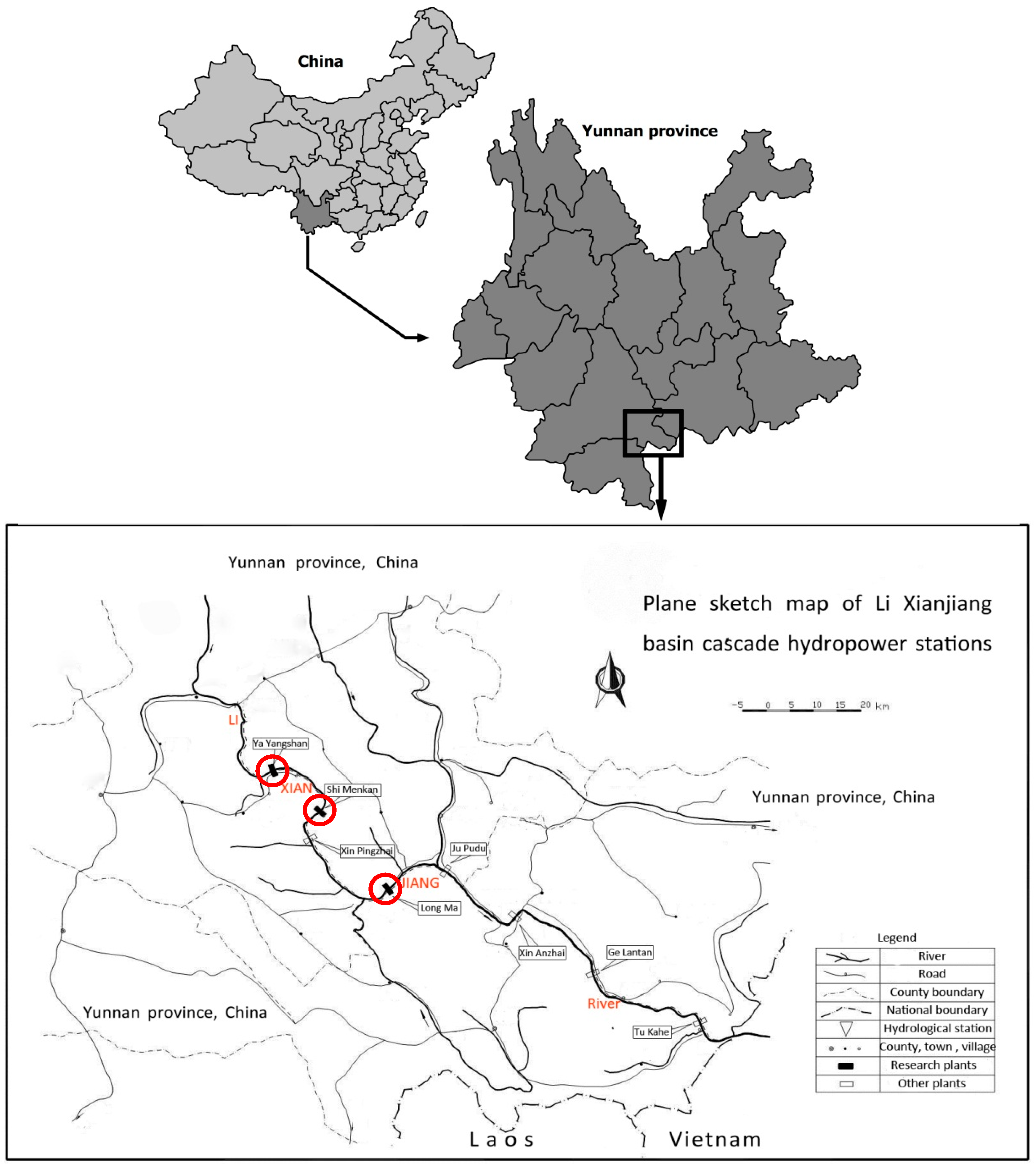
Li Xianjiang River is located in Yunnan Province of China, and it is a tributary of the Red River. Its main stream is 473 km in China, and its natural drop is about 1790 m. Its average annual runoff is approximately 460 m3/s at the border of China, and the control area is about 19,309 km2. There are seven hydropower stations on the main stream of Li Xianjiang river, i.e., Ya Yangshan, Shi Menkan, Xin Pingzhai, Long Ma, Ju Fudu, Ge Lantan, and Tu Kahe. Three hydropower stations, i.e., Ya Yangshan, Shi Menkan, and Long Ma, have the seasonal regulation performance, and they are thus selected as the research objects in this paper. The basic parameters of the selected hydropower stations are shown in Table 1, and their location in Li Xianjiang river basin is shown in Figure 2 [38].
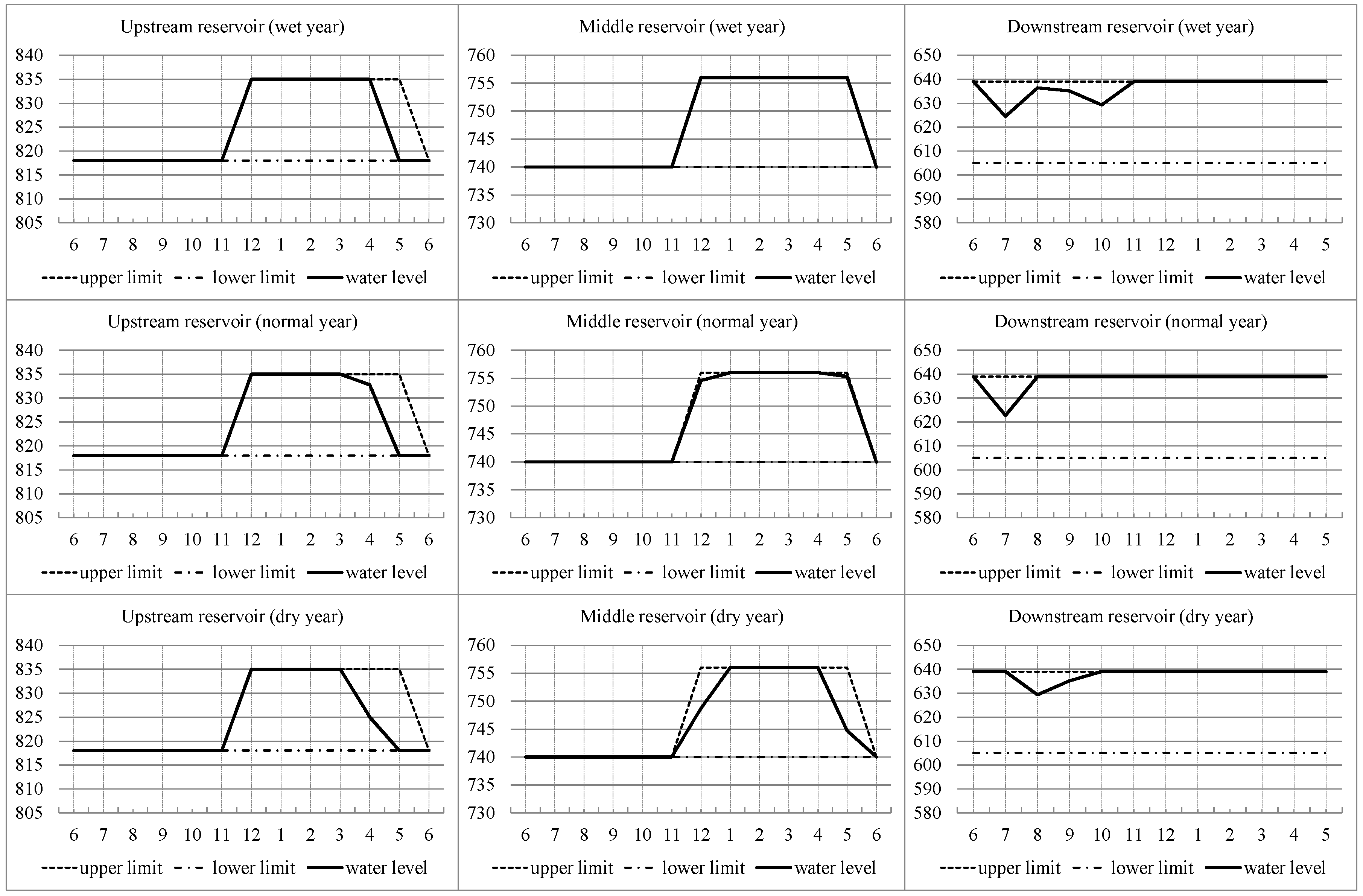
The available years of runoff data for this basin are from 1957 to 2000, a total of 43 years. According to the long series of runoff data, 1966, 1990 and 1988 are, respectively, selected as the wet year, normal year, and dry year in this paper. In order to obtain the optimal sample data for the extraction of operation rules, the first 35 years in the total 43 years are selected to implement the optimization calculation by MDP, and the last eight years in the total 43 years are selected as the inspection years to evaluate the performance of the extracted rules. Taking the three typical years as the representative, the water level variations of each reservoir are shown in Figure 3.
According to the above optimization results of cascade reservoirs by MDP, it can be found that the water level variations of each reservoir have a strong regularity. As we know, the output of reservoir depends on the amount of water and the water head, and the amount of water is determined by the climate conditions and has nothing to do with the dispatcher's operation. However, the water head is directly affected by the water level of reservoir, and the change of water level will directly lead to the change of output [39]. Therefore, when considering the strong regularity of water level variations in Figure 3, it is more convenient to take the water level as the decision variable to carry out the reservoir operation. According to Figure 3, the general operation rules for the water level variations of each reservoir are summarized as follows.
- (1)
- Regularity of the operation of upstream reservoir
① the water level is unchanged in the flood season, and the reservoir operates at the flood control level and generates the hydropower according to the natural inflow. ② the reservoir raises the water level to the normal water level at the end of the first stage of the non-flood season. ③ at the end of the non-flood season, the water of reservoir is released in advance for one or two stages, and the water level falls to the dead water level at the beginning of the last stage. At this moment, there is uncertainty about the number of stages (one or two) in which the water of reservoir released in advance. If the number of stages is two, then there is another uncertainty about the decrease degree of the water level in the first stage. ④ except for the stages in which the water of reservoir released in advance, the reservoir operation is maintained at the normal water level in the other stages of the non-flood season.
- (2)
- Regularity of the operation of middle reservoir
① the water level is unchanged in the flood season, and the reservoir operates at the flood control level and generates the hydropower according to the natural inflow. ② at the end of the first or the second stage of the non-flood season, the reservoir raises the water level to the normal water level, at this moment, there is uncertainty about the number of stages (one or two) in which the reservoir stores the water. If two stages are used to store water, then there is another uncertainty about the water level at the end of the first stage of the non-flood season. ③ at the end of the non-flood season, the water of reservoir is released in advance in some years, and these years corresponds to the years in which the water of upstream reservoir is released in advance for two stages. But, the reservoir is not necessarily to drop the water level to the dead water level at the beginning of the last stage, it may be at the end of the last stage. Therefore, there is uncertainty about the number of the stages (one or two) in which the water released in advance. If the last two stages are both involved in the water releasing, then there is uncertainty about the decrease degree of the water level in the first releasing stage. ④ except for the stages in which the water of reservoir released in advance and the stages used to store water, the reservoir operation is maintained at the normal water level in the other stages of the non-flood season.
- (3)
- Regularity of the operation of downstream reservoir
① the water level is fixed at the normal water level at the beginning of the first stage and at the end of last stage in the flood season, but the water level in the other stages of flood season varies greatly, and the uncertainty is relatively large. ② there is no stages to release water in advance in the non-flood season, and the reservoir operation is maintained at the normal water level.
4.2. Extraction of Operation Rules Based on the Optimal Results
Through the above summary and analysis to the regularity of the water level variations, it can be found that there are seven uncertain problems that need to be further studied: ① the number of the stages (one or two) in which the upstream reservoir’s water released in advance at the end of the non-flood season. ② the decrease degree of the water level in the first water releasing stage when two stages are used to release the upstream reservoir’s water in the non-flood season. ③ the number of water storage stages (one or two) of the middle reservoir at the beginning of the non-flood season. ④ the increase degree of the water level in the first water storage stage when the middle reservoir takes two stages to store water at the beginning of the non-flood season. ⑤ the number of the stages (one or two) of the middle reservoir to release water at the end of the non-flood season. ⑥ the decrease degree of the water level in the first water releasing stage when the middle reservoir takes two stages to release water at the end of the non-flood season. ⑦ the variations of the water level of downstream reservoir in the flood season, except for at the beginning of the first stage and the end of last stage. If the above seven uncertain problems are transformed into deterministic problems, the operation processes of the cascade reservoirs can be determined uniquely, and this operation processes are consistent with the optimal results by MDP.
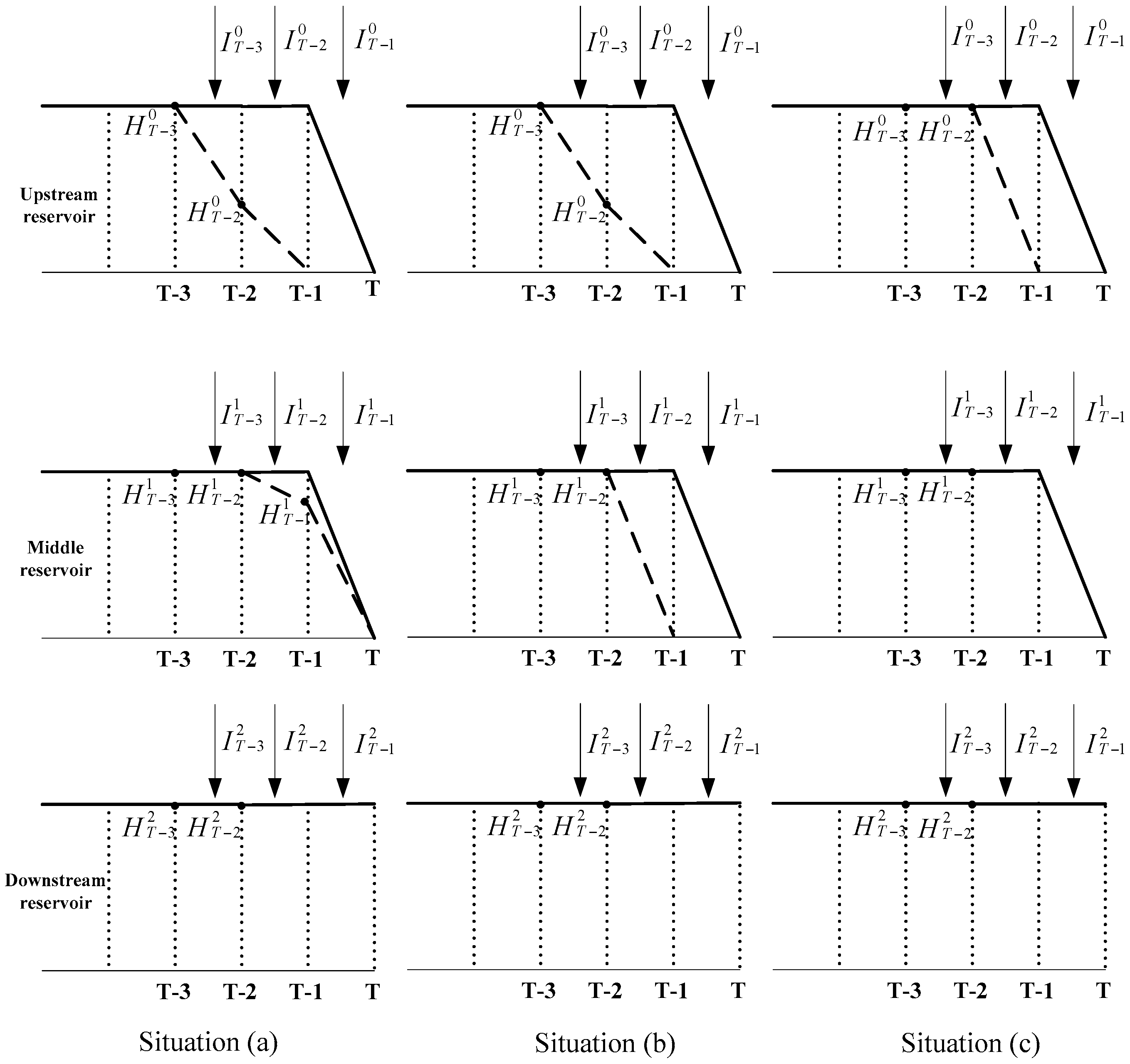
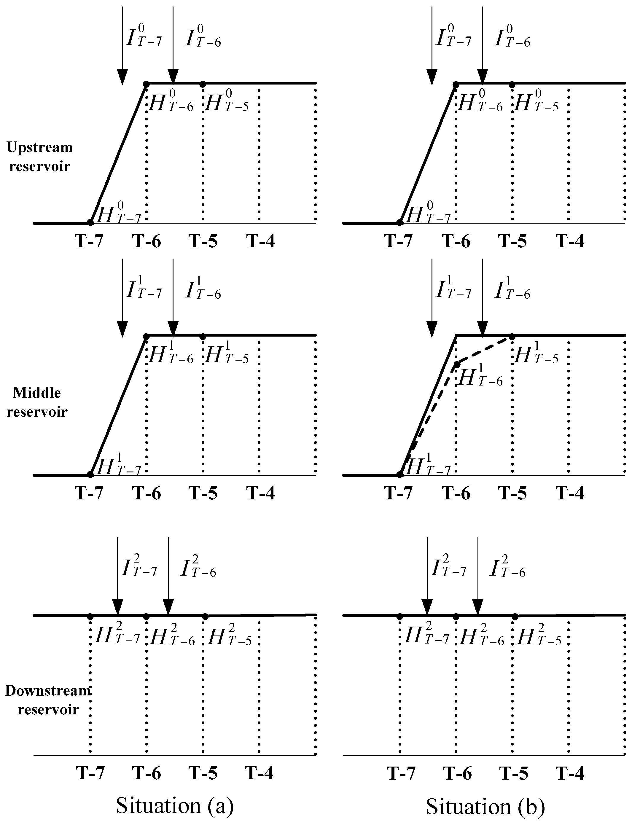
For the above uncertain problems ①, ②, ⑤, and ⑥, three situations can be summarized: (a) the water of upstream and middle reservoirs released in advance for two stages. (b) the water of upstream reservoir released in advance for two stages, but the water of middle reservoir released in advance for one stage. (c) the water of upstream reservoir released in advance for one stage, and the water of middle reservoir do not released in advance.
The above three situations are shown in Figure 4. The affected stages of situation (a) is the last three stages of non-flood season, and the uncertain variables are two water levels, the first one is the water level at the beginning of the penultimate stage of upstream reservoir in the non-flood season, and the second one is the water level at the beginning of the last stage of middle reservoir in the non-flood season, i.e., and , in Figure 4. The affected stages of situation (b) is also the last three stages of non-flood season, but the uncertain variable is only the water level at the beginning of the penultimate stage of upstream reservoir in the non-flood season, i.e., in Figure 4. The affected stages of situation (c) are the last two stages of non-flood season, and there is no uncertain variable. Thus, it can be concluded that the maximum number of affected stages of the three situations is three, and the number of uncertain variables are at most two. Because the three affected stages are all located at the back of the entire operation period, and the water level of each reservoir before the three affected stages in the non-flood season is determined, a sub-model of the operation optimization of cascade reservoirs can be established to solve and , and to solve the uncertain decision problems for the three affected operation stages in the non-flood season. Taking the maximum power generation as the goal, the objective function of the sub-model for the last three operation stages of non-flood season can be established, as follows.
where E3 is the maximum sum of the power generation of the three affected stages. The constraints of the sub-model are shown in Figure 4 and Section 2.2 (i.e., Formulas (3) to (7)). The inflow of the (T − 3)th, (T − 2)th, and (T − 1)th stage, which are IT−1, IT−2 and IT−3, can be obtained by the forecasting when solving the sub-model. By discretizing the water level and in their feasible range, the optimal value of and and the total power generation of the three affected stages can be determined by searching for all of the discretized combinations of and . When considering the limitation of forecasting conditions, the inflow of the (T − 2)th and (T − 1)th stage can be replaced by their multi-year average values in the optimization calculation.
For the uncertain problems ③ and ④, two situations can be summarized: (a) the middle reservoir raises the water level to normal water level in the first stage of the non-flood season. (b) the middle reservoir raises the water level to the normal water level in the first two stages of the non-flood season.
The above two situations are shown in Figure 5. The affected stage of situation (a) is the first stage of non-flood season, and there is no uncertain variable. The affected stages of situation (b) are the first two stages of non-flood season, and the uncertain variable is the water level of the middle reservoir at the end of the first stage in the non-flood season, i.e., in Figure 5. Thus, from the above analysis, it can be concluded that the maximum number of affected stages of the two situations is two, and the number of uncertain variable is only one. Because the water levels of each reservoir before and after the two affected stages are both fixed, a sub-model of the operation optimization of cascade reservoirs can be established to solve , and to solve the uncertain decision problems for the first two affected stages of non-flood season. Taking the maximum power generation as the goal, the objective function of the sub-model for the first two stages of non-flood season can be established, as follows.
where E2 is the maximum sum of the power generation of the first two stages in the non-flood season. The constraints of the sub-model are shown in Figure 5 and Section 2.2 (i.e., Formulas (3) to (7)). The solving process of this sub-model is similar to the sub-model for the last three stages of non-flood season. Similarly, when considering the limitation of forecasting conditions, the inflow of the (T − 6)th stage can be replaced by its multi-year average value in the optimization calculation.
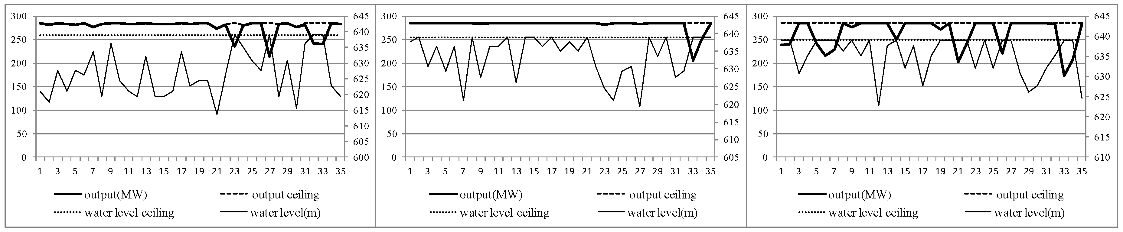
For the uncertain problem ⑦, the regularity of water level variations of downstream reservoir is not obvious in flood season except for the first stage and the last stage, i.e., July, August, and September. So, we cannot directly get the operation rules for these stages. However, in contrast, the regularity of the output processes of these stages are clear and strong. Through the comparison and analysis between the water level variations and the output variations, it can be found that the output of each stage is basically equal to the expected output when the initial water level does not reach the normal water level, especially in July and August, as shown in Figure 6. When the water level reach the normal water level, the high water level should be maintained in the operation as long as there is no water abandonment, and make sure that the output is not less than the guaranteed output. Therefore, the operation rules of downstream reservoir in July, August and September can be summarized as follows: If the water level at the beginning of the stage is lower than the normal water level, the reservoir operates with the expected output in this stage. If the water level at the beginning of the stage is equal to the normal water level, then the high water level can be maintained while trying to avoid water abandonment in the operation. When the reservoir is maintaining at the high water level, the forecasted inflows of the current and the next stages are necessary to avoid water abandonment.
After the above seven uncertain problems are solved, the whole operation period of each reservoir can be divided into four characteristic sections (section A, B, C, and D), according to the regularity of operation, then the operation rules of each section are proposed respectively, and then the operation rules of each reservoir for the whole operation period can be established after an integration, as shown in Table 2. Because the obtained operation rules are basically consistent with the optimization results by MDP, and it has a certain of global optimality, so it can be directly used to guide the actual operation of cascade reservoirs in the Li Xianjiang basin.
4.3. Discussion and Analysis of Simulation Results
Taking the runoff of the inspection years as the input, this paper implements the operation simulation of Li Xianjiang cascade reservoirs based on the extracted operation rules. The comparison of the annual power generation between the extracted operation rules and MDP is shown in Table 3, and the comparison of the annual power generation between the extracted operation rules and the conventional joint operation method is shown in Table 4. The guarantee rate of output of MDP is 87%, and there is little difference between the operation rules and conventional joint operation method on that, and they are both around 81%. The conventional joint operation method shown in Table 4 refers to the operation of cascade hydropower stations based on the existing single reservoir operation curves.
From Table 3, it can be seen that, for the simulation results of the extracted operation rules, there is a large gap compared with the optimization results of MDP. The annual power generations of operation rules are all less than that of MDP in the wet year, normal year, dry year, and the inspection years. The difference is between 2% and 4%, and the guarantee rate of output of the extracted operation rules is reduced by 6% when compared with MDP. However, as compared with the conventional joint method in Table 4, the annual power generations of operation rules are both improved in the inspection years and the three typical years, which increased by 0.7%, 0.4%, 2.3%, and 1.7%, respectively, and their guarantee rates of output are basically the same. Therefore, in general, the operation rules that are extracted in this paper have a certain of rationality and guiding significance. Furthermore, the extracted operation rules are obtained based on the optimal sample data of MDP, and they are the general summary of the regularity of reservoir operation. Especially the principle of “the upstream reservoir releases the water in advance at the last few stages of the whole operation period, so that to make full use of the high water head of downstream reservoirs to generate more electricity before it drops down”, included in the operation rules has great significance to guide the actual operation of cascade reservoirs, and this is consistent with the basic principle of water storage and supply of reservoir, and reflects the consistency of actual facts with the operation rules. Hence, the rationality of the extracted operation rules in this paper is further proved.
5. Conclusions
In order to make full use of the hydraulic and water relationship between the upstream and downstream reservoirs, and give full play to the role of compensative regulation, and to improve the economic benefits and water resources utilization efficiency of cascade reservoirs, this paper takes Li Xianjiang cascade reservoirs as an example to extract and evaluate operation rules, the following conclusions are summarized.
- (1)
- In this paper, the MDP model of cascade-reservoir operation optimization was proposed, and the MDP successfully realized its effective application in the optimization of cascade reservoirs. Based on the optimal sample data, the general regular information of each reservoir in each operation stage was summarized and extracted, and seven uncertain problems over the whole operation period of cascade systems were summarized.
- (2)
- In order to solve the uncertain problems of cascade system during the operation period, this paper proposed two sub-models, i.e., sub-model for the last three stages of non-flood season and sub-model for the first two stages of non-flood season. The two sub-models successfully solved the water storage operation problem of middle reservoir at the beginning of the non-flood season, and the water discharge problem of upstream and downstream reservoirs at the end of the non-flood season. The operation rules of each reservoir were finally extracted by dividing the whole operation period into four characteristic sections.
- (3)
- When comparing the simulation results of the extracted rules with those of conventional joint operation method, it was found that the power generation of the proposed rules had a certain degree of improvement both in inspection years and typical years, and the increase is 0.7%, 0.4%, 2.3%, and 1.7%, respectively. The guarantee rate of output was basically unchanged. So, on the whole, the operation rules extracted in this paper have the practical value, and they can be used to guide the actual operation of Li Xianjiang cascade reservoirs.
However, the difference is still large when compared with the optimal results of MDP, which indicates that there are some shortcomings in the extracted operation rules. The possible reason is that the inflow of some future stages is replaced by its multi-year average value in solving the two sub-models, which may lead to some errors. Moreover, the research of operation rules extraction in this paper mainly aimed at the Li Xianjiang cascade reservoirs, so the universality of the proposed method needs more case studies or some kind of benchmarking with previous studies to verify, and this is what the authors are going to do next.
Acknowledgments
This study was financially supported by National Key R&D Program of China (2017YFC0405900), the CRSRI Open Research Program (Program SN: CKWV2016371/KY), the Natural Science Foundation of China (91647114) and the Fundamental Research Funds for the Central Universities (HUST: 2017KFYXJJ 198 and HUST: 2016YXZD047). The authors are grateful to the anonymous reviewers for their comments and valuable suggestions.
Author Contributions
Z.J. and H.Q. conceived and designed the experiments; W.W. and Y.Q. performed the experiments; Z.J. analyzed the data and results; Z.J. and H.Q. wrote the paper.
Conflicts of Interest
The authors declare no conflict of interest.
References
- Yüksel, I. Hydropower for sustainable water and energy development. Renew. Sustain. Energy Rev. 2010, 14, 462–469. [Google Scholar] [CrossRef]
- Li, F.; Qiu, J. Multi-objective optimization for integrated hydro-photovoltaic power system. Appl. Energy 2016, 167, 377–384. [Google Scholar] [CrossRef]
- Gebretsadik, Y.; Fant, C.; Strzepek, K.; Arndt, C. Optimized reservoir operation model of regional wind and hydro power integration case study: Zambezi basin and South Africa. Appl. Energy 2016, 161, 574–582. [Google Scholar] [CrossRef]
- George, C. Feasibility study of a hybrid wind/hydropower-system for low-cost electricity production. Appl. Energy 2002, 72, 599–608. [Google Scholar]
- Lu, D.; Wang, B.; Wang, Y.; Zhou, H.; Liang, Q.; Peng, Y.; Roskilly, T. Optimal operation of cascade hydropower stations using hydrogen as storage medium. Appl. Energy 2015, 137, 56–63. [Google Scholar] [CrossRef]
- Kangrang, A.; Chaleeraktrakoon, C. Genetic algorithms connected simulation with smoothing function for searching rule curves. Am. J. Appl. Sci. 2007, 4, 73–79. [Google Scholar] [CrossRef]
- Jiang, Z.Q.; Sun, P.; Ji, C.M.; Zhou, J.Z. Credibility theory based dynamic control bound optimization for reservoir flood limited water level. J. Hydrol. 2015, 529, 928–939. [Google Scholar] [CrossRef]
- Chang, F.; Chen, L.; Chang, L. Optimizing the reservoir operating rule curves by genetic algorithms. Hydrol. Process. 2005, 19, 2277–2289. [Google Scholar] [CrossRef]
- Taghian, M.; Rosbjerg, D.; Haghighi, A.; Madsen, H. Optimization of conventional rule curves coupled with hedging rules for reservoir operation. J. Water Resour. Plan. Manag. 2014, 140, 693–698. [Google Scholar] [CrossRef]
- Ding, Y.; Tang, D.; Meng, Z. A new functional approach for searching optimal reservoir rule curves. Adv. Mater. Res. 2014, 915–916, 1452–1455. [Google Scholar] [CrossRef]
- Chang, F.; Lai, J.; Kao, L. Optimization of operation rule curves and flushing schedule in a reservoir. Hydrol. Process. 2003, 17, 1623–1640. [Google Scholar] [CrossRef]
- Afshar, A.; Emami Skardi, M.; Masoumi, F. Optimizing water supply and hydropower reservoir operation rule curves: An imperialist competitive algorithm approach. Eng. Optim. 2015, 47, 1208–1225. [Google Scholar] [CrossRef]
- Ak, M.; Kentel, E.; Savasaneril, S. Operating policies for energy generation and revenue management in single-reservoir hydropower systems. Renew. Sustain. Energy Rev. 2017, 78, 1253–1261. [Google Scholar] [CrossRef]
- Chang, J.; Li, Y.; Yuan, M.; Wang, Y. Efficiency evaluation of hydropower station operation: A case study of Longyangxia Station in the Yellow River, China. Energy 2017, 135, 23–31. [Google Scholar] [CrossRef]
- Eum, H.; Kim, Y.; Palmer, R.N. Optimal drought management using sampling stochastic dynamic programming with a hedging rule. J. Water Resour. Plan. Manag. 2010, 137, 113–122. [Google Scholar] [CrossRef]
- Shokri, A.; Haddad, O.B.; Marino, M.A. Reservoir operation for simultaneously meeting water demand and sediment flushing: Stochastic dynamic programming approach with two uncertainties. J. Water Resour. Plan. Manag. 2013, 139, 277–289. [Google Scholar] [CrossRef]
- Kangrang, A.; Lokham, C. Optimal reservoir rule curves considering conditional ant colony optimization with simulation model. J. Appl. Sci. 2013, 13, 154–160. [Google Scholar] [CrossRef]
- Chu, W.; Yang, T.; Gao, X. Comment on “High-dimensional posterior exploration of hydrologic models using multiple-try DREAM (ZS) and high-performance computing” by Eric Laloy and Jasper A. Vrugt. Water Resour. Res. 2014, 50, 2775–2780. [Google Scholar] [CrossRef]
- Yang, C.; Chang, L.; Yeh, C.; Chen, C. Multi-objective planning of surface water resources by multi-objective genetic algorithm with constrained differential dynamic programming. J. Water Resour. Plan. Manag. 2007, 133, 499–508. [Google Scholar] [CrossRef]
- Zhu-Ge, Y.; Xie, P. The application of DDDP method to optimal operation for cascade reservoirs based on state transformation matrix. In Proceedings of the 2010 International Conference on Computational and Information Sciences ICCIS, Chengdu, China, 17–19 December 2010; pp. 76–80. [Google Scholar]
- Lu, B.; Li, K.; Zhang, H.; Wang, W.; Gu, H. Study on the optimal hydropower generation of Zhelin reservoir. J. Hydro-Environ. Res. 2013, 7, 270–278. [Google Scholar] [CrossRef]
- Mathlouthi, M.; Lebdi, F. Use of generated time series of dry events for the optimization of small reservoir operation. Hydrol. Sci. J. 2009, 54, 841–851. [Google Scholar] [CrossRef]
- Pereira, M.V.F.; Pinto, L.M.V.G. Multi-stage stochastic optimization applied to energy planning. Math. Program. 1991, 52, 359–375. [Google Scholar] [CrossRef]
- Zhang, R.; Zhou, J.; Zhang, H.; Liao, X.; Wang, X. Optimal operation of large-scale cascaded hydropower systems in the upper reaches of the Yangtze River, China. J. Water Resour. Plan. Manag. 2014, 140, 480–495. [Google Scholar] [CrossRef]
- Momtahen, S.; Dariane, A.B. Direct search approaches using genetic algorithms for optimization of water reservoir operating policies. J. Water Resour. Plan. Manag. 2007, 133, 202–209. [Google Scholar] [CrossRef]
- Arnel, G.; Aleš, Z. Short-term combined economic and emission hydrothermal optimization by surrogate differential evolution. Appl. Energy 2015, 141, 42–56. [Google Scholar]
- Ji, C.; Yu, S.; Zhou, T.; Yang, Z.; Liu, F. Application of ant colony algorithm for hydropower dispatching function optimization. Autom. Electr. Power Syst. 2011, 35, 103–107. [Google Scholar]
- Hormwichian, R.; Kangrang, A.; Lamom, A. A conditional genetic algorithm model for searching optimal reservoir rule curves. J. Appl. Sci. 2009, 9, 3575–3580. [Google Scholar] [CrossRef]
- Mensik, P.; Starý, M.; Marton, D. Water management software for controlling the water supply function of many reservoirs in a watershed. Water Resour. 2015, 42, 133–145. [Google Scholar] [CrossRef]
- Helseth, A.; Fodstad, M.; Askeland, M.; Mo, B.; Nilsen, O.B.; Pérez-Díaz, J.I.; Chazarra, M.; Guisández, I. Assessing hydropower operational profitability considering energy and reserve markets. IET Renew. Power Gener. 2017, 11. [Google Scholar] [CrossRef]
- Ma, C.; Lian, J.; Wang, J. Short-term optimal operation of Three-gorge and Gezhouba cascade hydropower stations in non-flood season with operation rules from data mining. Energy Convers. Manag. 2013, 65, 616–627. [Google Scholar] [CrossRef]
- Yuan, W.; Wu, Z. Discussion on application of cooperative coevolution of differential evolution algorithm to optimal operation of cascaded reservoirs. J. Hydroelectr. Eng. 2012, 31, 39–43. [Google Scholar]
- Raso, L.; Schwanenberg, D.; van de Giesen, N.C.; van Overloop, P.J. Short-term optimal operation of water systems using ensemble forecasts. Adv. Water Resour. 2014, 71, 200–208. [Google Scholar] [CrossRef]
- Zhang, Y.; Jiang, Z.; Ji, C.; Sun, P. Contrastive analysis of three parallel modes in multi-dimensional dynamic programming and its application in cascade reservoirs operation. J. Hydrol. 2015, 529, 22–34. [Google Scholar] [CrossRef]
- Jiang, Z.; Qin, H.; Ji, C.; Feng, Z.; Zhou, J. Two dimension reduction methods for multi-dimensional dynamic programming and its application in cascade reservoirs operation optimization. Water 2017, 9, 634. [Google Scholar] [CrossRef]
- Ji, C.M.; Jiang, Z.Q.; Sun, P.; Zhang, Y.K.; Wang, L.P. Research of multi-dimensional dynamic programming based on multi-layer nested structure and its application in cascade reservoirs. J. Water Resour. Plan. Manag. 2015, 141, 1–13. [Google Scholar] [CrossRef]
- Nandalal, K.D.W.; Bogardi, J.J. Dynamic Programming Based Operation of Reservoirs: Applicability and Limits; Cambridge University Press: Cambridge, UK, 2007. [Google Scholar]
- Jiang, Z.; Li, A.; Ji, C.; Qin, H.; Yu, S.; Li, Y. Research and application of key technologies in drawing energy storage operation chart by discriminant coefficient method. Energy 2016, 114, 774–786. [Google Scholar] [CrossRef]
- Yang, G.; Guo, S.; Liu, P.; Xu, C. Multiobjective reservoir operating rules based on cascade reservoir input variable selection method. Water Resour. Res. 2017, 53, 3446–3463. [Google Scholar] [CrossRef]
Figure 1.
Reverse recursion calculation diagram of Multi-dimensional Dynamic Programming (MDP).

Figure 2.
The location of the selected hydropower stations in Li Xianjiang River basin.

Figure 3.
The water level variations of each reservoir in three typical years.

Figure 4.
Sub-model for the last three stages of the non-flood season.

Figure 5.
Sub-model for the first two stages of the non-flood season.

Figure 6.
The water level and output variations of downstream reservoir in many years.


Table 1.
Parameters of the three hydropower stations in Li Xianjiang basin.
| Items | Unit | Ya Yangshan | Shi Menkan | Long Ma |
|---|---|---|---|---|
| Normal water level | m | 835 | 756 | 639 |
| Dead water level | m | 818 | 740 | 605 |
| Total storage volume | 108 m3 | 3.08 | 1.75 | 5.1 |
| Regulation volume | 108 m3 | 1.34 | 0.82 | 3.34 |
| Storage factor | -- | 0.035 | 0.02 | 0.056 |
| Regulation performance | -- | season | season | season |
| Design assurance rate | % | 95 | none | 95 |
| Guaranteed output | MW | 23.2 | 33.5 | 61.2 |
| Annual power generation | GWh | 499 | 573 | 1284 |
| Water head loss coefficient | 10−5 | 8.658 | 5.28 | 2.642 |
| Maximum head loss | m | 5.59 | 2.33 | 3 |
| Integrated efficiency coefficient | -- | 8.3 | 8.3 | 8.3 |
| Flood control level | m | 818 | 740 | none |
| Flood season | month | 6~10 | 6~10 | none |
Table 2.
Operation rules of cascade reservoirs in the four characteristics sections.
| Reservoir | Upstream Reservoir | Middle Reservoir | Downstream Reservoir |
|---|---|---|---|
| Segmentation diagram |  |  |  |
| Section A | Operating at the flood control level in flood season | Operating at the flood control level in flood season | Operating with output ceiling when water level is below normal level, and trying to keep high water level and not to abandon water when water level is equal to normal level |
| Section B | Operating with the sub-model for the first two stages of the non-flood season | Operating with the sub-model for the first two stages of the non-flood season | Maintain the normal water level operation |
| Section C | Maintain the normal water level operation | Maintain the normal water level operation | Maintain the normal water level operation |
| Section D | Operating with the sub-model for the last three stages of the non-flood season | Operating with the sub-model for the last three stages of the non-flood season | Maintain the normal water level operation |
Table 3.
Comparison of power generation between the extracted rules and MDP (unit: GWh).
| Year | Simulation Results by Rules (1) | MDP (2) | Decrement [(2) − (1)]/(1) |
|---|---|---|---|
| Multi-year average | 2323 | 2392 | 3.0% |
| Wet year | 2710 | 2816 | 3.9% |
| Normal year | 2214 | 2263 | 2.2% |
| Dry year | 1822 | 1888 | 3.6% |
Table 4.
Comparison of power generation between the extracted rules and conventional method (unit: GWh).
Table 4.
Comparison of power generation between the extracted rules and conventional method (unit: GWh).
| Year | Simulation Results by Rules (1) | Conventional Joint Operation (2) | Increment [(1) − (2)]/(1) |
|---|---|---|---|
| Multi-year average | 2323 | 2307 | 0.7% |
| Wet year | 2710 | 2699 | 0.4% |
| Normal year | 2214 | 2164 | 2.3% |
| Dry year | 1822 | 1792 | 1.7% |
© 2017 by the authors. Licensee MDPI, Basel, Switzerland. This article is an open access article distributed under the terms and conditions of the Creative Commons Attribution (CC BY) license (http://creativecommons.org/licenses/by/4.0/).
Share and Cite
MDPI and ACS Style
Jiang, Z.; Qin, H.; Wu, W.; Qiao, Y. Studying Operation Rules of Cascade Reservoirs Based on Multi-Dimensional Dynamics Programming. Water 2018, 10, 20. https://doi.org/10.3390/w10010020
AMA Style
Jiang Z, Qin H, Wu W, Qiao Y. Studying Operation Rules of Cascade Reservoirs Based on Multi-Dimensional Dynamics Programming. Water. 2018; 10(1):20. https://doi.org/10.3390/w10010020
Chicago/Turabian StyleJiang, Zhiqiang, Hui Qin, Wenjie Wu, and Yaqi Qiao. 2018. "Studying Operation Rules of Cascade Reservoirs Based on Multi-Dimensional Dynamics Programming" Water 10, no. 1: 20. https://doi.org/10.3390/w10010020
Note that from the first issue of 2016, this journal uses article numbers instead of page numbers. See further details here.