Non-Point Source Nitrogen and Phosphorus Assessment and Management Plan with an Improved Method in Data-Poor Regions

1
State Key Laboratory of Simulation and Regulation of Water Cycle in River Basin, China Institute of Water Resources and Hydropower Research, Beijing 100038, China
2
College of Hydrology and Water Resources, Hohai University, Nanjing 210098, China
*
Author to whom correspondence should be addressed.
Water 2018, 10(1), 17; https://doi.org/10.3390/w10010017
Submission received: 21 November 2017
/
Revised: 10 December 2017
/
Accepted: 21 December 2017
/
Published: 26 December 2017
Abstract
:To enhance the quantitative simulation and integrated assessment of non-point source (NPS) pollution in plateau lakes in data-poor regions, a simple and practical NPS assessment method is developed by combining the improved export coefficient model (ECM) and the revised universal soil loss equation (RUSLE). This method is evaluated via application to the Chenghai Lake watershed (Yunnan Province, China), which contains a typical plateau lake. The estimated results reflect the actual situation within the watershed. The total nitrogen (TN) and total phosphorus (TP) loads in the study area in 2014 were 360.35 t/a (44.30% dissolved nitrogen (DN) and 55.70% adsorbed nitrogen (AN)) and 86.15 t/a (71.40% adsorbed phosphorus (AP)), respectively. The southern and eastern portions of the watershed are key regions for controlling dissolved and adsorbed pollutants, respectively. Soil erosion and livestock are the main TN and TP pollution sources in the study area and should be controlled first. Additionally, reasonable and practical suggestions are proposed to minimize water pollution according to a scenario analysis. The method in this study provides a foundation for scientific theories that can be used in water resources protection planning and the method can be applied to the NPS assessment of similar regions with scarce data.
1. Introduction
Problems related to the pollution of water in river basins because of rapid economic development and population growth have become increasingly prominent. Various types of industrial and agricultural activities have placed unprecedented pressure on the aquatic environment [1,2,3]. Moreover, people have placed new and higher requirements on the living environment, given the progress of science and technology and the increase in standards of living, especially in terms of water quality [4]. In recent years, non-point source (NPS) pollution has become the primary cause of water pollution; in contrast, point source (PS) pollution has been gradually controlled [5]. Large loads of sediment, nitrogen (N) and phosphorus (P) are discharged into water bodies, contributing to increases in suspended solids and toxic and hazardous substances, reductions in dissolved oxygen and water eutrophication [6]. This process both disturbs the balance of the original ecosystem and affects normal human life, thus threatening human health [7]. At present, the large quantities of the nutrients N and P that result from NPS pollution (NPS-N and NPS-P, respectively) cause serious hydrological and environmental issues worldwide and have become the predominant obstacle to the protection of the aquatic environment [8]. Agricultural NPS pollution is one of the most important factors affecting surface water quality in North America [9]. The U.S. Environmental Protection Agency (USEPA) has estimated that 53% of the 27% assessed miles of rivers and streams and 69% of the 45% assessed acreage of lakes, ponds and reservoirs in the nation are severely affected by NPS pollution [10]. Additionally, 64% of the N input and 46% of the P input to the North Sea originate from diffuse sources, of which agriculture is the dominant source [11]. Agriculture causes 60% and 40–50% of the emissions of total nitrogen (TN) and total phosphorus (TP), respectively, to surface waters in the Netherlands [12]. NPS pollution (which is mainly agricultural) produces 94% of the riverine N loading and 52% of the riverine P loading in the aquatic environment in Denmark [13]. In China, the First National Survey of Pollution Sources Bulletin shows that emissions of N and P resulting from agricultural activities account for 57% and 67% of the total amounts of these pollutants, respectively [14]. In addition, China, as an agricultural county, has been a primary user of fertilizer and pesticide [15]. The water quality compliance rate of rivers, lakes and the ocean is 65%, 42% and 78%, respectively, even if point source pollution is fully controlled, according to research results from the United States, Japan and other countries [16]. Therefore, NPS pollution has surpassed PS pollution as a cause of lake eutrophication and water quality deterioration and has gradually become a major pollution source around the world [17]. Today, many countries recognize the dangers of NPS pollution and numerous studies regarding the control of NPS pollution have been carried out. The eco-environmental protection plan contained in China’s 13th Five-Year Plan (2016–2020) demonstrates a clear focus on the comprehensive management of the agricultural environment in rural areas and the control of agricultural NPS pollution. However, China is still developing NPS pollution control technologies and the relevant monitoring campaigns are very expensive and conspicuous; therefore, constructing a functional database of runoff quality is quite difficult, especially in areas where the monitoring network is characterized by a lack of discharge gauging stations [18]. An NPS pollution load estimation system must be established to guide the control of NPS pollution [19]. Thus, the identification and quantification of NPS characteristics is a reasonable basis for protecting the water environment of river basins [20]. Such investigations have both important scientific significance and practical significance in the control of NPS pollution.
In the 1960s, many investigations showed that the terminal management technology traditionally used to control PS pollution had difficulties controlling NPS pollution effectively. Many scholars then began conducting quantitative research on NPS pollution. With the emergence of “3S” technologies, such as GIS, NPS pollution models have developed rapidly and have become extremely effective quantitative tools for the simulation and estimation of NPS pollution. Currently, NPS evaluation models can be divided into physically based models and empirical models. The physically based models include Agricultural Runoff Management Model (ARMM) [21], Chemical Runoff and Erosion from Agricultural Management System (CREAMS) [22], Areal Non-point Source Watershed Environment Response Simulation (ANSWERS) [23], Agricultural Non-point Source Pollution Model (AGNPS) [24], Hydrological Simulation Program-Fortran (HSPF) [25], Simulator for Water Resources in Rural Basins (SWRRB) [26] and Soil and Water Assessment Tool (SWAT) [27]. Such models both quantify the amounts of NPS pollutants produced and simulate the attenuation and transformation of these pollutants during the transfer process. To date, physically based models have been used in numerous studies. However, due to the complexity of the required model input and parametric uncertainty, none of the existing physically based models is widely applicable in simulating NPS pollutants in practical applications, especially in most developing countries [28]. However, the use of physically based models has also led to practical outcomes, such as the development of empirical models [29]. Empirical models utilize the black box principle to avoid the complex processes associated with the behavior of NPS pollution. Such models have advantages in that they require few inputs and are simple to operate, even when long time series of monitoring data are lacking for particular watersheds of interest [19]. Empirical models can both guarantee the accuracy of the simulation results and reflect the variation characteristics of different types of NPS pollutants. Based on their migration behavior, NPS pollutants can largely be grouped into two classes, dissolved and adsorbed. The export coefficient model (ECM) is considered to be reliable for the estimation of dissolved NPS pollutants [30]. The earliest ECM was proposed by the United States and Canada [31,32] and was used to explore the response of lake eutrophication to land-use changes in the early 1970s. This work provided a new concept for researchers in the quantification of NPS pollution, although this model has considerable limitations in that it assumes that the export coefficients of all land-use types are equal. To address the shortcomings of the initial ECM, many scholars have improved this model and these improvements have greatly advanced the development of this method. A remarkably advanced ECM was developed by Johnes that improves the accuracy of evaluation and prediction [33]. The ECM has been greatly improved in terms of both the choice of nutrient sources and its sensitivity to land-use change. The ECM is widely applied; for example, Mattikalli et al. analyzed the pollutants N and P in the Glen River Basin in the UK and simulated their changes under multiple scenarios [34]. S. Shrestha et al. used water quality data to evaluate the export coefficients of pollution sources and constructed a watershed-scale ECM to explore the NPS pollution load in the Fuji River [35]. Ding et al. improved the ECM to analyze the spatial distribution of nutrient loads in the upper reach of the Yangtze River [36]. Mattikalli et al., S. Shrestha et al. and Ding et al. all found that the ECM is still an effective tool for assessing NPS pollution loads due to the lack of long-term observational time series for model calibration in many practical applications. Adsorbed pollutants are typically attached to soil microparticles, which act as migration carriers and their production is largely controlled by soil erosion. The adsorbed pollutants produced by soil erosion represent pollution emissions. The revised universal soil loss equation (RUSLE) represents a new generation of soil erosion prediction models and was developed by the United States Department of Agriculture (USDA) based on the universal soil loss equation (USLE) in 1997 [37]. It predicts erosion rates in ungauged watersheds based on watershed characteristics and local hydro-climatic conditions [38] and assesses the spatial heterogeneity of soil erosion. Veljko Perović et al. evaluated soil erosion rates and their spatial distribution in the hilly, mountainous Nisava River basin in southeastern Serbia using the RUSLE in combination with remote sensing (RS) data [39]. Fu et al. used the RUSLE and a geographic information system (GIS) to assess soil losses on the Loess Plateau of China [40]. With the development of GIS and RS techniques, the RUSLE has been widely used in the quantitative assessment of soil erosion worldwide and it is considered to be an effective technical method for soil and water conservation planning. Note that the empirical model has several deficiencies; for example, the ECM and the RUSLE establish a direct relationship between nutrient inputs and outputs and they do not sufficiently consider the mechanisms and processes by which NPS pollution occurs [19]. The existing ECM is suitable for regions where the precipitation and terrain are homogenous. Given that it does not consider variations in precipitation or topography, the ECM cannot be applied to regions with uneven precipitation distributions or varied and complex terrain [41]. In carrying out watershed loss calculations, previous studies have used regional average values and do not consider the effects of distance and terrain. Therefore, it is crucial to compensate for these shortcomings and to develop empirical models to represent regional characteristics and obtain more accurate results. The focus of this paper is to improve the ECM and the RUSLE and to increase the range of their applicability.
Lake Chenghai is one of nine major plateau lakes on the Yunnan Plateau in southwestern China and is one of only three lakes in the world where Spirulina is found naturally. Lake Chenghai occupies an extremely prominent position in the social and economic development of the region. However, in recent years, due to the impact of human activities and limited water exchange, the lake has experienced serious problems, including eutrophication and water shortages. In addition, the Lake Chenghai watershed experiences some of the most serious soil erosion in Yunnan Province. The climate of the Lake Chenghai watershed is dry and features limited rain and intense evaporation; these conditions are related to the elevation of the lake, which is situated at 1501 m a.s.l. and its proximity to the typically hot and dry Jinsha River valley. The calculation of NPS pollutant loads for Lake Chenghai is challenging because, compared with the patterns in other regions, the transport of NPS pollutants is relatively strongly controlled by precipitation and terrain and no long-term monitoring datasets exist. The following questions thus arise. How can the pollution sources of Lake Chenghai be quantified? Which pollution sources should receive priority for control measures? Considerable research work has been conducted on these issues from different perspectives. For example, Zou et al. simulated the fate and transport of TN and TP in the Lake Chenghai watershed using a two-dimensional model of hydrodynamics and water quality [42]. Dong et al. analyzed the characteristics of the distribution of P and the various forms of P in Lake Chenghai using field-based measurements [43]. Zhou et al. established a mass conservation model to calculate the reference conditions of TP and TN [44]. However, these studies partly neglect the pollutant loads discharged into the lake and very few researchers have analyzed the pollutant loads discharged into Lake Chenghai in detail. Based on these considerations, in this paper, a methodology that attempts to overcome the lack of monitoring data is developed to make up for the research gap in the Lake Chenghai watershed. Additionally, a study on this topic should provide an opportunity to identify the predominant pollution sources and provide a reasonable plan for NPS pollution control.
The predominant objectives of this study are (1) to develop a simple and practical method of NPS pollution assessment for use in regions with scarce data; (2) to analyze the spatial variations in and the apportionment of NPS-N and NPS-P; and (3) to discuss reductions in the quantities of TN and TP discharged into Lake Chenghai under different scenarios. The NPS load estimation method proposed by this study based on the improved ECM and RUSLE provides a new means to study NPS pollution in data-poor regions. The method is simple, systematic and universal, thereby expanding the application range of NPS pollution assessments.
2. Materials and Methods
2.1. Study Site
Lake Chenghai is situated between 26°27′ N and 26°28′ N and between 100°38′ E and 100°41′ E in Yunnan Province in southwestern China. It is a typical closed lake in the transitional zone between the Qinghai-Tibetan Plateau and the Yunnan-Guizhou Plateau and has an elevation of 1852.58 m (Figure 1). The Lake Chenghai watershed has a total area of 318.3 km2, an average lake area of 73.45 km2 (1960–2016) and contains a population of 33,603 (2014). The watershed experiences a typical subtropical highland monsoon climate. From 1960 to 2016, the average annual precipitation in the watershed was 740.90 mm and the annual evaporation was 2040.3 mm, resulting in a shortage of water resources. Eighty-five percent of the annual precipitation occurs from June to October. The watershed contains 37 rivers with a total length of 395 km; most of these rivers are seasonal. The vegetation coverage of the watershed is 47% and this coverage has been severely reduced by excessive deforestation. The Lake Chenghai watershed has been divided into 29 sub-basins through field investigations and river network generalization. Given the rapid increase in economic development, abundant nutrients have been transported into the lake, resulting in severe eutrophication and algal blooms in Lake Chenghai. Therefore, load evaluations and source apportionments of NPS-N and NPS-P at the watershed scale are necessary to offer a reference for NPS pollution control and the protection of the aquatic environment.
2.2. Description and Preprocessing of the Data Sets
Taking into account the availability and completeness of the relevant data, we focus on the analysis of the discharge of NPS pollutants into Lake Chenghai in 2014. The primary data sets used in this study are as follows. (1) A land-use map with a resolution of 30 m interpreted from Landsat 8 OLI images collected in 2014 was obtained from the Geospatial Data Cloud, Computer Network Information Centre, Chinese Academy of Sciences (http://www.gscloud.cn). The remote sensing images were interpreted using the ENVI software package, version 4.8 (Harris Corporation, Melbourne, FL, USA). (2) A vegetation cover map with a spatial resolution of 250 m was established from NDVI [45] values extracted from the MOD13Q1 product provided by the National Aeronautics and Space Administration (NASA). (3) A soil type database and soil map with a spatial resolution of 100 m were provided by the Institute of Soil Science, Chinese Academy of Sciences. (4) Precipitation data (2006–2016) collected at three stations in and near the watershed were obtained from the China Meteorological Administration and the local bureau of meteorology. The precipitation data were interpolated using the inverse distance weighting (IDW) method to determine the precipitation over the Lake Chenghai watershed. (5) A digital elevation model (DEM) with a resolution of 30 m was obtained from the Institute of Geographical and Natural Resources Research, Chinese Academy of Sciences. (6) Data on the rural population, fecal pollution and livestock within the study area were obtained from the Statistical Year Book. Every factor within the ECM and the RUSLE is calculated using the ArcGIS software package, version 10.2.2 (Redlands, CA, USA, Environmental Systems Research Institute). The spatial resolution of all of the raster data sets is set to 100 m and these data sets are projected into the Albers Equal Area Conic projection.
Because different land-use types often yield different pollutants, we classify the land uses in Lake Chenghai into six categories, namely woodlands (FRST), grasslands (PAST), farmlands (AGRL), water bodies (WATR), barren lands (BARR) and built-up areas (URLD). To enable greater detail, the farmland areas are divided into dry lands, paddy fields and orchards. Moreover, the woodland areas include forests, open forests and shrublands (Figure 1b). A field campaign performed by the research team verified that the classification results meet the accuracy requirements. From the perspective of the spatial distribution reflected by the land-use map, woodlands make up the largest fraction of the watershed (39.6% of the total area), whereas farmlands and grasslands are the second and third most abundant land-use types, representing 15.19% and 14.83% of the total area, respectively.
In the soil map, the soil types are classified into seven categories (Figure 1c) following the soil classification criteria of the China Soil Database [46]. The spatial distribution shown on the soil map indicates that red soils, cinnamon red soils and red limestone soils dominate the Lake Chenghai watershed and together account for 92.71% of the total land area. These soil types, which are located around Lake Chenghai, are vulnerable to the effects of water erosion because of their composition and structure [47]. Other soil types occupy smaller portions of the region and occur in high mountain areas.
2.3. Model Description
Dissolved pollutants are usually transported by rainfall to water bodies and are produced mainly by land-use practices, the rural population and livestock; they are represented in the improved ECM. The adsorbed pollutants caused by soil erosion can be calculated using the RUSLE.
where W is the total pollution load (t a−1); Wdis is the dissolved pollution load (t a−1); and Wads is the adsorbed pollution load (t a−1).
2.3.1. Improved ECM
Precipitation and terrain represent critical intrinsic elements that influence NPS pollution [48]. Therefore, it is imperative to add representations of precipitation and terrain to the ECM. A version of the ECM that considers precipitation and terrain factors is likely to be more suitable for the evaluation of NPS pollution in plateau lakes [36,49]. The pollutant loading of a given basin is calculated according to the scale of the sub-basins. The improved ECM is expressed as follows:
where L is the loss of nutrients (t a−1); n is the number of spatial unit i, which is set to be 100 m × 100 m; m is the type of nutrient source j, which includes land-use, livestock and rural population; αi is the precipitation impact factor of spatial unit i; βi is the terrain impact factor of spatial unit i; Eij is the export coefficient for nutrient source j (t (km2 a)−1 or kg (ca a)−1) in spatial unit i; Aij is the area of land-use (km2), the number of livestock, or the number of people in spatial unit i; and Pi is the input of nutrients from atmospheric deposition of spatial unit i (t a−1). Due to the lack of corresponding monitoring data, this study does not consider the atmospheric deposition of nutrients.
1. Precipitation impact factor α
Previous studies indicate that precipitation intensity and duration have significant effects on the timing of peak nutrient concentrations and the annual losses of nutrients, respectively [50]. In addition, most of the dissolved pollutants delivered into Lake Chenghai are carried by runoff and the runoff, in turn, is mainly affected by precipitation in Chenghai watershed. Thus, a functional relationship exists between the nutrient losses produced by NPS pollution and rainfall. The precipitation impact factor αi is considered in terms of the temporal impact factor αit and the spatial impact factor αis of spatial unit i. The temporal impact factor αit can be calculated by assessing the correlation relationship between annual precipitation and the pollutant loads discharged into the lake. The spatial impact factor αis is the ratio of precipitation within a spatial unit to the mean precipitation in the watershed as a whole. Combining αit with αis yields αi, which can be expressed as follows:
where f(ri) is the correlation relationship between the annual rainfall, ri, in spatial unit i (mm) and the annual load of dissolved pollutants discharged into the lake (t) in a given year. f(rave) is the correlation relationship between the multi-annual mean rainfall, rave, in the watershed as a whole (mm) and the multi-annual mean dissolved pollutant load discharged into the lake (t). Ri is the annual rainfall in spatial unit i and Rave is the mean rainfall received by the watershed as a whole in a given year (mm).
As stated previously, we first established a correlation between the annual precipitation r and the dissolved nitrogen (DN) and phosphorus (DP) contents of the pollutant loads delivered into Lake Chenghai. Due to reliable observations of the dissolved pollutant loads delivered into Lake Chenghai are lacking. Thus, in this study, we used some results about dissolved pollutant loads delivered into Lake Chenghai from 1980 to 2010 presented by Zhou et al. [44]. The correlation relationship between the annual rainfall r and the annual load of dissolved pollutants discharged into the lake L can be expressed as follows:
where LDN is the annual load of DN discharged into the lake (kg) and LDP is the annual load of DP discharged into the lake (kg).
Figure 2 illustrates the trends in annual precipitation from 1985 to 2016. A trend test reveals that the mean annual precipitation shows a decreasing trend over the past 32 years. The magnitude of the trend in mean annual precipitation in the Lake Chenghai watershed from 1985 to 2016 is −19.26 mm/10 years. In this study, abrupt changes in mean annual precipitation are identified using Mann-Kendall techniques. Between 1985 and 2016, an abrupt change in mean annual precipitation occurs in 2006 (p < 0.05) (Figure 3). This result is consistent with that reported by Wang et al. [51]. The precipitation impact factor α and the rainfall erosivity factor R in the following discussion are calculated from 2006 to 2016, according to the results of the abrupt change test.
The multi-year average rainfall received by the Lake Chenghai watershed from 2006 to 2016 is 702.47 mm. The calculated multi-year average rainfall can be substituted into Equation (4) to determine the multi-annual mean pollutant loads of DN and DP discharged into the lake. With the addition of the spatial impact factor of rainfall, the rainfall impact factor αi for DN and DP can be expressed as follows:
The calculated values of the precipitation impact factor αiDN range from 0.83 to 0.88 in 2014, whereas the αiDP values range from 0.79 to 0.90 in 2014 (Figure 4a,b).
2. Terrain impact factor β
The ECM considers the area of and export from different land use types; however, it does not take the inhomogeneity of the underlying surface into consideration. In addition to land use types, the terrain of the underlying surface has a significant effect on the dissolved pollutants associated with NPS pollution. Slope gradient and length are two important terrain metrics and the former is more important than the latter for NPS pollution. Therefore, we mainly consider the spatial inhomogeneity of slope gradient in the improved ECM. Runoff plays an important role as a carrier of dissolved pollutants and the slope gradient determines the losses of dissolved pollutants by influencing the amount of runoff. Correlation studies confirm that pollution loads and slope gradients are positively correlated with runoff. Thus, the influence of slope on dissolved pollutants transforms the relationship between slope gradient and runoff [52]. Some scholars have demonstrated that runoff can be described as a power function of the slope gradient multiplied by a constant [53]. The nonuniformity of the concentrations of dissolved pollutants caused by variations in the slope gradient is reflected by the ratio of the slope within a spatial unit to the average slope of the whole watershed. The terrain impact factor β is expressed as follows:
where L(θi) is the pollution load within spatial unit i and L(θave) is the pollution load of the entire watershed. θi is the slope gradient for spatial unit i (100 m × 100 m); θave is the average slope gradient of the whole watershed; and d is a constant.
The values of d in Equation (13) are confirmed by the results of the study of Zhang et al. [54]. The average slope gradient of the whole watershed is calculated to be 13.30° and the terrain impact factor β is expressed as follows:
The calculated values of the terrain impact factor β range from 0.00 to 2.34. The distribution of β includes high values to the west and low values to the east (Figure 4c). This spatial distribution is almost the same as the geographic characteristics of the Chenghai watershed. The western portion of this region contains deep valleys and steep slopes, whereas the eastern portion contains relatively gentle slopes and the southern portion is flat.
3. Export coefficients
There are four sources of DN and DP in the Chenghai Lake watershed: the rural population, livestock, land use and soil erosion. Considering the shortage of regional monitoring data and the cost in terms of the time required to collect such data, we performed a literature review to determine the values of the export coefficients for the different land use types considered in this study. Eight watersheds from the existing literature have been selected based on their proximity to the Chenghai Lake watershed and the presence of hydrological and climatic conditions that are similar to those of the Chenghai Lake watershed. The export coefficients of the different land use types in the Chenghai Lake watershed have been estimated based on the mean values of the results from these eight watersheds. Furthermore, the export coefficients are modified based on short-term storm runoff plot experiments. Table 1 shows the cited export coefficients of the different land-use types and the values determined in this study.
Additionally, the export coefficients for the rural population and livestock are determined from the pollution source census of Yunnan province. According to the related research results, dissolved pollutants from soil erosion account for 8% of the adsorbed pollutants. The export coefficients for each pollution source in the Chenghai Lake watershed are listed in Table 2.
4. The estimated pollution loads discharged into the lake
Note that the simulated results of the improved ECM are pollutant yields and do not consider the processes of artificial collection, physical deposition or chemical reactions during transport; thus, not all of the pollutants produced reach the outlet of the watershed. To verify the accuracy of the pollutant loads simulated using the improved ECM, we employ the rate of pollutant loading into the lake λr to convert the pollutant yields into pollution loads discharged into the lake. Moreover, the vertical and horizontal distances between each grid cell and the outlet of the catchment are different, so the degree to which the dissolved pollutants are attenuated during the migration process also varies. The weighting modifies the average pollutant loss rate into Lake Chenghai and the distances and elevation differences between the grid cells and the outlet of the catchment are used to obtain more accurate estimates of the pollution loads discharged into the lake. The formula that describes the relationship between pollutant yields and the pollution loads discharged into the lake is as follows:
where Lr is the pollutant load discharged into the lake (t a−1); λr is the loss rate of pollutants into the lake; and L is the pollutant yield of NPS pollution (t). The collection and disposal rates of domestic sewage, domestic waste, fecal discharge and livestock waste are 20%, 80%, 45% and 45%, respectively. Considering the types of drainage channels and temperature, the average ratio of pollutant discharge into the lake from Majun and Xingyi are 0.9 and those of the other villages are 1.0. In this study, the ratios of DN and DP discharged into the lake from the different land-use types are 0.3 and 0.2, respectively, as confirmed by previous studies [65].
5. Comparing the simulated values with the monitoring data
Because this study improves the Johnes ECM through accounting for precipitation, slope, the distances between pollution sources and water bodies and other relevant factors, it is essential to examine the accuracy of the improved ECM by comparing the simulated values with the observational data. The relative error Re is used to evaluate the accuracy of the simulation results via the process of verification. The calculation formula for Re is as follows:
where Re is the relative error of the simulation; Rt represents a simulated value; and Qt is the corresponding observation.
At present, the research on NPS pollution in the Chenghai Lake watershed is in its initial stages and historical data, especially observations of water quality before 2009, are relatively scarce. The scarcity of this data increases the difficulty of verification. Therefore, for the case mentioned above and the purposes of this study, we obtained estimates of the DN and DP discharged into the lake in 2010 (706.5 mm), 2012 (686.5 mm) and 2014 (715.0 mm) from the local environmental protection department to evaluate the accuracy of the simulation results; these three years are all normal flow years. An analysis of the relative error between the simulated results produced by the improved ECM and the observed data is shown in Figure 5. The simulated DN values agree well with the observed data and the relative error is within 10%, which indicates that the improved ECM simulates DN reasonably well. In contrast, the relative error associated with DP is relatively large, approximately 30%. However, relatively little DP is discharged into the lake; thus, the absolute differences are relatively small. These findings demonstrate that the improved ECM provides a more accurate simulation of DN loads than DP loads. One reason for this difference is that the DN loads simulated by the improved ECM are relatively sensitive. Additionally, NPS-P mainly exists in the adsorbed state and the improved ECM has some limitations in the estimation of DP.
2.3.2. The RUSLE
Adsorbed nitrogen and phosphorus (AN and AP, respectively) are transported through soil erosion. In this study, we use the RUSLE empirical model to predict the annual losses. Using the RUSLE, the amounts of AN and AP discharged into the lake can be calculated using the following equation:
where Wads is the adsorbed pollutant load discharged into the lake (t a−1) and λads is the transition ratio of the soil, which is a key factor that affects the adsorbed pollutant loads discharged into the lake. The average ratio of soil loss into the lake for the whole watershed has been reported to be 0.28 [66]. Considering that the distance and the elevation difference between each spatial unit and the outlet of the catchment differ, the amount of soil erosion also varies. The weighting modifies the average transition ratio of the soil by using the distance and the elevation difference between each grid cell and the outlet of the catchment to obtain a more accurate estimate of the eroded soil discharged into the lake. Here, u represents a given land use type (km2); Xu is the average soil loss from land use type u caused by soil erosion, which can be calculated using Equation (19) (t a−1); Au is the area of land use type u (km2); Cs is the background mass fraction of N or P in the soil (%), which can be obtained from the soil database of the Second Soil Survey of China; and η is the accumulation ratio of N or P in the soil, which can be derived from the literature [44]. The accumulation ratios of N and P are 1.35 and 1.28, respectively.
The RUSLE is the most extensively used soil erosion model at present because it has a simple form and the meaning of each factor is clear. The RUSLE is expressed as follows:
Here, R is the rainfall erosivity factor (MJ mm ha−1 h−1 year−1), which quantifies the dynamics of soil separation and transport caused by rainfall and in this study, the monthly rainfall data from 2006 to 2016 for the study area are used to determine the average annual value of R based on Wischmeier and Smith (1978) [67]. Ku is the soil erodibility factor (t ha h ha−1 MJ−1 mm−1); it represents the rate of soil loss per rainfall erosion index unit, as measured on a standard plot and it is often determined using inherent soil properties, such as soil texture, organic matter content, permeability and other factors [68]. In this study, the values of Ku are estimated using the methods described in the EPIC model introduced by Williams [69]. L, S, C and P are dimensionless. LS is calculated by multiplying the length factor L by the steepness factor S and this product reflects the ratio of soil erosion losses from the slope of the study area to the soil erosion losses from a standard runoff plot. The length and steepness factors of the slope are determined from the DEM of the Chenghai Lake watershed in the GIS environment. In this study, the length factor L is calculated using an empirical formula [70]. The maximum slope gradient considered by the RUSLE model is 18%, whereas 82.01% of the area of the Chenghai Lake watershed has slope gradients exceeding 18%. Therefore, in this study, we use separate equations based on McCool et al. (1987) [71] and Liu et al. (2000) [72] for slopes with gradients that are less than and greater than 18%, respectively. Cu is the land cover and management practice factor and Pu is the conservation support practice factor. Cu and Pu represent factors that inhibit soil erosion and primarily reflect the influence of vegetation, crops and management practices on soil erosion. Cu is calculated using the mathematical relationship between slope, sediment yield and vegetation coverage and Pu is determined from the land use map, field surveys and other relevant information. The values of these factors range from near zero for well-covered land or areas where effective conservation practices are in place to one for barren areas or areas where no conservation practices have been implemented.
The rainfall erosivity factor (R), the soil erodibility factor (Ku), the slope length factor (LS), the cover and management practice factor (Cu) and the management practice factor (Pu) are represented on a raster grid with 100 m × 100 m spatial units in the GIS environment. LS, Cu and Pu are dimensionless. We then use the Map Algebra function in the GIS environment to multiply all of the factors to obtain the average annual soil loss. According to the results of the RUSLE, the average annual soil loss from the whole watershed is 2384 t km−2, which is very close to the value obtained from Jing et al. (2315 t km−2) [73]. With the RUSLE, the estimated loads of AN and AP in this study are 200.7 t a−1 and 61.6 t a−1, respectively. Compared with the results of 197.9 t a−1 and 66.0 t a−1 for AN and AP, respectively, from the literature review [74], the relative errors in AN and AP are 1.89% and −6.74%, respectively. These results demonstrate that the estimation model of adsorbed pollutant loads discharged into the lake is consistent with the actual situation.
2.4. Calculation of the Amounts of NPS Pollutants
The flowchart shown in Figure 6 summarizes all of the input data and the specific calculation procedures used in this study. After the computational methods and calculation results of each factor in the modified ECM and the RUSLE have been described and analyzed, DN and DP can be obtained using the improved ECM and AN and AP can be determined using the RUSLE. We can then assess the variations in the TN and TP discharged into the lake from NPS pollution in the Chenghai Lake watershed.
3. Results
3.1. Estimating DN and DP
3.1.1. Land Use
Many nutrients, particularly those produced due to unreasonable land use practices and including DN and DP, affect the survival of aquatic organisms and change the balance in aquatic ecosystems. Thus, it is essential to identify the DN and DP characteristics associated with different land-use types. The DN and DP produced by a land-use type represent the pollution emissions. Unused nitrogen and phosphorus fertilizer in the dissolved state in the soil are washed down to stream channels. A subsequent series of physical sedimentation and chemical reaction processes in the stream channel determines the amount discharged into the lake. The simulated DN and DP loads discharged into the lake and their intensities are shown in Table 3. The DN and DP loads and their intensities display obvious differences among the different land-use types. Agricultural lands (dry lands, paddy fields and orchards) make the largest contributions to the pollutant loads discharged into the lake, followed by woodlands (forests, open forests and shrublands) and grasslands. Agricultural lands also have the largest intensities, followed by barren lands and grasslands. The average DN load discharged into the lake due for each land use is 5.8 t a−1. The land-use type that is the primary source of DN is dry land, which makes the largest contributions (17.6 t a−1) and accounts for 30.19% of the total, followed by grasslands (10.2 t a−1, 17.49%) and forests (10.2 t a−1, 17.42%). The value for paddy fields is also higher than the mean value for the watershed as a whole (which is estimated to be 7.9 t a−1) and paddy fields contribute 13.49% of the total. The average DN intensity for the whole watershed is 0.28 t (km2 a)−1; the intensities of orchards, dry lands, paddy fields and barren lands all exceed the mean value for the watershed as a whole. The DP load and intensity for the various land-use types are generally similar to those of the DN but differ slightly. The average DP load discharged into the lake due to land use is 0.6 t a−1. Dry land is also the major contributor among all of the land-use types; it makes the largest contribution (1.9 t a−1) and accounts for 31.49% of the total, followed by grasslands (1.3 t a−1, 21.53%). The contributions from paddy fields and forests show slight differences between DN and DP; paddy fields contribute slightly larger amounts of DP (14.06%) than DN (13.49%) but the proportional contribution of DP (12.41%) from forests is substantially smaller than that of DN (17.42%). The average intensity of DP among the different land-use types is 0.03 t (km2 a)−1; as with DN, the intensities of DP in orchards, dry lands, paddy fields and barren lands all exceed the mean value of the watershed as a whole.
DN and DP show similar spatial distributions (Figure 7); the regions with DN and DP loads discharging into the lake due to land use are mainly distributed in the southern and northern portions of the watershed (where the cumulative contribution percentages from land use are 70.32% and 72.23% for DN and DP, respectively), followed by the eastern and western portions of the watershed. The main reason for this observation is that agricultural production is relatively high in the southern and northern portions of the watershed (the agricultural lands in these regions represent 54.87% and 19.37% of the total area of agricultural lands in the watershed) and very large amounts of chemical fertilizers are applied to the farmland. However, woodlands and grasslands are concentrated in the eastern and western portions of the watershed, so the pollutant loads discharged into the lake from these areas are relatively low.
3.1.2. The Rural Population and Livestock
Increases in consumption by modern people and improvements in their dietary structure have increased the demand for meat and milk products. These developments have stimulated the development of animal husbandry. The large amounts of excreta produced result in an enormous potential ecological crisis. Therefore, it is important to analyze the pollution loads generated by livestock and the rural population. After artificial treatment, the pollution loads generated by livestock and the rural population represent pollution emissions and the pollution emissions undergo a series of physical sedimentation and chemical reaction processes in the stream channel before being discharged into the lake. Figure 8 illustrates the DN and DP loads discharged into the lake by the rural population and livestock. The average DN and DP loads discharged into the lake by the rural population are 32.6 t a−1 and 5.5 t a−1, respectively. Specifically, the manure emissions from the rural population represent the largest contributions of DN and DP, for which the cumulative contribution percentage is 130.18%, followed by domestic garbage (38.50%) and domestic sewage (31.32%). Moreover, the average DN and DP loads discharged into the lake by livestock are 52.6 t a−1 and 8.1 t a−1, respectively. In terms of spatial distribution, the regions with the largest DN and DP contributions produced by the rural population and livestock are mainly distributed in the southern and northern portions of the watershed. These areas contain the majority of the population (79.33% of the total population) and the livestock (77.74% of the total livestock population). This distribution results in high levels of livestock manure emissions, domestic garbage and sewage. For comparison, the proportions of the population and livestock in the eastern and western portions of the watershed are relatively small; thus, the pollution loads discharged into the lake from these areas are relatively low.
3.1.3. DN and DP Loads Discharged into Lake Chenghai
Figure 9 illustrates the spatial distribution of DN and DP loads discharged into the lake from the individual sub-watersheds. Comparing DN and DP, we find that the distribution of DN is similar to that of DP but that differences in their spatial distributions are obvious. The DN loads discharged into the lake from the individual sub-watersheds range from 1.0 t a−1 to 19.2 t a−1, whereas the DP loads range from 0.2 t a−1 to 2.9 t a−1. Both of these quantities reach their maxima in sub-watersheds No. 7 and No. 20 in the southern part of the study region; the cumulative contributions from these sub-watersheds are 23.61% and 23.28%, respectively. The DN and DP loads discharged into the lake from different regions in 2014 are shown in Table 4. The total DN load discharged into the lake is much larger than the total DP load. The total DN and DP loads discharged into the lake from the watershed as a whole are 158.5 t a−1 and 24.7 t a−1, respectively. Note that the DN and DP from the southern part of the study area account for 49.51% and 50.16% of the total amounts, respectively. Obviously, to limit the discharges of dissolved pollutants, control measure should first be implemented in the southern portion of the watershed.
3.2. Estimating AN and AP
3.2.1. Loads of AN and AP Discharged into Lake Chenghai
The estimated loads of AN and AP discharged into the lake from the different regions are shown in Table 5. In terms of the contribution percentages, the eastern part of the study area is the predominant contributor (39.38%) of AN, followed by the northern (24.57%), southern (22.27%) and western (13.78%) portions of the study area. The eastern, southern, northern and western portions of the watershed are the main contributors of AP and these regions are associated with contribution percentages of 39.20%, 25.12%, 21.69% and 13.99%, respectively. To gain a deeper understanding of the discharges of AN and AP, we also examine the spatial distribution of AN and AP at the scale of individual sub-watersheds (Figure 10). The spatial distributions of AN and AP are quite similar. They both display high values in the eastern portion of the study area, especially in sub-watersheds No. 1 and No. 28, for which the cumulative contribution percentages are 15.99% and 16.14%, respectively. Thus, control measures should be implemented first in the eastern portion of the watershed to limit the discharge of adsorbed pollutants. The AN loads discharged into the lake from individual sub-watersheds range from 1.2 to 17.2 t a−1, whereas the AP loads range from 0.4 to 5.3 t a−1. The total AN and AP loads discharged into the lake from the watershed are 200.7 and 61.6 t a−1, respectively.
3.2.2. Spatial Distribution Characteristics
Adsorbed pollutants are caused by multiple factors that interact with each other. The analysis of the relationship between the losses of adsorbed pollutants and their driving factors is of great significance in identifying optimal management practices for controlling NPS pollution. Based on the statistical functions of the GIS package, we estimate the loads and intensities of AN and AP for the different land-use types, slope gradients and slope aspects in the study area. The aim is to identify the regions with high loads and intensities of adsorbed pollutants. According to the results of the calculations discussed above, the mean pollution intensity values for AN and AP for the entire watershed are 0.83 and 0.25 t/km2, respectively.
The loads and intensities of AN and AP discharged into the lake are closely related to land use and they display obvious differences among areas with different land-use types (Figure 11). Because they cover a relatively large area, woodlands are associated with the maximum loads of AN and AP (115.9 and 36.4 t/a) in terms of total amounts, followed by grasslands (44.0 and 13.4 t/a). From the perspective of AN and AP intensities, barren lands (1.18 and 0.30 t/km2), forests (0.91 and 0.29 t/km2) and grasslands (0.94 and 0.28 t/km2) all exceed the mean pollution intensities for the watershed as a whole. The barren lands within the Chenghai Lake watershed represent the land-use type with the highest intensities. These areas suffer serious soil erosion because of poor site conditions, the presence of edaphic barrens and other factors. These characteristics result in the pollution load intensity of the barren lands being the largest, although the area of barren lands corresponds to only 3.53% of the total area of the watershed. Because the woodlands are mostly natural secondary forests with low forest coverage and because the grasslands contain single-species communities and display sparse vegetation coverage, they do not slow the loss of adsorbed pollutants. Of the seven land-use types, barren lands, forests and grasslands display the highest AN and AP intensities and should be prioritized for control measures.
To enable the comprehensive implementation of soil and water conservation, a general planning rule, GB/T 15772–2008, has been issued by the General Administration of Quality Supervision, Inspection and Quarantine of the People’s Republic of China and the Standardization Administration of the People’s Republic of China. The AN and AP associated with regions of different slope gradients in 2014 are presented in Figure 12. The results indicate that the loads and intensities of AN and AP have a positive relationship with the slope gradient. Approximately 68% of the AN and AP losses occurred on slopes with gradients exceeding 15°. Additionally, nearly 35% of the AN and AP losses occurred in regions with slopes exceeding 25°. The reason for this positive relationship between adsorbed pollutants and the slope gradient could be that farmland and built-up areas occupy a major proportion (59.94%) of the areas with gradients below 5° and human activities reduce the impacts of soil erosion to some extent. Second, rapid vegetation growth and relatively high vegetation coverage tend to slow the process of soil erosion. In contrast, in regions with slopes exceeding 25°, higher runoff rates are associated with stronger soil erosion and topographic conditions favoring intense soil erosion develop. Note that the intensities of forests, grasslands, farmlands and barren lands are obviously affected by the slope gradient; compared to these four land-use types, built-up areas exhibit a less evident increasing trend in intensity. Based on the analysis described above, conservation tillage measures, such as contour tilling and terraced ploughing, should be practiced on farmlands situated on slopes with gradients exceeding 25°. In addition, it is necessary to strengthen the management of barren lands.
4. Discussion
4.1. Source Analysis and Pollution Loads for TN and TP
Synthesizing the DN, DP, AN and AP loads, we obtain the simulated TN and TP values of the watershed as a whole for 2014. The TN load is much higher than the TP load. The TN load, which accounts for the influences of land-use types, livestock, the rural population and soil erosion, is 360.3 t/a. Of this amount, DN makes up 159.6 t/a, which corresponds to a proportional contribution of 44.30% and AN makes up 200.7 t/a, which corresponds to a proportional contribution of 55.70%. The total load of TP is 86.2 t/a; DN and AP contribute 24.6 and 61.6 t/a, which correspond to proportional contributions of 28.56% and 71.44%, respectively. Obviously, the contributions of DN and AN are essentially identical in terms of TN, whereas TP occurs mainly in the form of AP. Based on the N:P ratio, we can provide a reliable assessment of which nutrient is the limiting factor for algae growth in Lake Chenghai. The TN:TP ratio is 4.18 and the DN:DP ratio is 6.49. Based on the optimal N:P ratios complied by Havens et al. [75], it is expected that Lake Chenghai will be nitrogen-limited in the future, especially during the summer and the wet season. This finding is consistent with the results of previous studies by Zou et al. [76].
The average intensity for DN is 0.67 t/km2, whereas that of DP is 0.11 t/km2. The Chenghai Lake watershed drains into the Yangtze River, which is the largest river in China. The average DN and DP intensities in the upper reach of the Yangtze River were estimated to be 1.96 t/km2 and 0.09 t/km2 by Ding et al. [36], which are higher and lower, respectively, than the values reported in the present study. The main reason for this phenomenon is that the dominant land-use type within the watershed studied by Ding et al. is agricultural lands, whereas the dominant land-use types in the Chenghai Lake watershed are woodlands and grasslands, which played some role in the mitigation and retention of DN and DP. Moreover, statistically, the use of P fertilizer per unit area is 75.09 t/km2 in the Chenghai Lake watershed, which is higher than the national average; at present, the average utilization percentage of P fertilizer in China is 10~20% [77]). The improper use of N and P fertilizer will lead to serious losses of P fertilizer. In addition, 37.3% of the dry land is distributed in areas with relatively steep terrain (>15°), aggravating the loss of P fertilizer. The average intensities of AN and AP are 0.83 and 0.25 t/km2, respectively. Considering the results reported for the upper reach of the Yangtze River by Shen et al. [49], the average AN and AP are estimated to be 0.30 t/km2 and 0.14 t/km2, respectively, which are lower than those obtained in the present study. A major reason for these differences is that the Chenghai watershed experiences some of the most severe soil and water degradation in Yunnan Province and approximately 61.59% of the watershed is slightly or heavily eroded. Note that the background levels of soil nutrients are relatively high [44].
To gain a deeper understanding of the composition of NPS pollution in the Chenghai Lake watershed, we also examine the source apportionment for TN and TP. The results are shown in Figure 13. The predominant source of TN is soil erosion, which accounts for 55.70% of the total; livestock represents the second largest source (14.59%). Of the land-use types present in the catchment, farmlands, which include dry lands, paddy fields and orchards, account for 7.08% and the other land-use types contribute a total of 9.12%. The rural population accounts for the portion of the nutrient loading contributed by human activities and is associated with a TN contribution of 9.05%. The lowest contribution, only 4.46%, is derived from the dissolved part of the eroded soil. The predominant sources of TP are ranked differently from those of TN. Soil erosion is still the most important source (71.36%) and its contribution percentage for TP is significantly higher than that for TN. Soil erosion is followed by livestock (9.41%) and the rural population (6.37%). Because the P pollution is mainly carried by soil particles, the amount of DP associated with the process of soil erosion is correspondingly higher; the associated contribution is 5.72%. Of the land-use types, farmland accounts for 3.84% of the TP, whereas the other land-use types contribute 3.22%.
Considering the factors that together affect the TN and TP loads, the cumulative contribution percentages of TN and TP are as follows: soil erosion (127.14%), livestock (24.00%), the rural population (15.42%), other land-use types (12.96%), farmlands (10.29%) and the dissolved parts of the eroded soil (10.17%). Therefore, soil erosion and livestock are the main sources of pollution that influence TN and TP in the Chenghai Lake watershed. These sources should clearly be controlled first.
4.2. Measures of NPS Pollution
4.2.1. Regional Divisions for NPS Pollution Control
The Chenghai Lake watershed is divided into a conservation region, a control region and a repair region, according to land use intensity, ecological suitability and fragility and the distribution of topography and villages. The information shown in Table 6 and Figure 14 describes the spatial characteristics of the regional divisions for NPS pollution management.
4.2.2. Measures for NPS Pollution Control
Compared with other empirical models, the method established by this study is based on the raster scale for statistical data, taking into account the artificial treatment rate of NPS pollution. The λr and λads have been revised. Therefore, the evaluation results more closely reflect the actual situation in terms of the amount of emissions and the amount discharged into the lake. Based on these results, we set up typical scenarios to evaluate the reduction effects of NPS pollution control measures. The scenario analysis both assesses the influence of various management strategies on water quality [78] and enables the selection of the best management practices for the implementation of total maximum daily loads (TMDLs) [79]. According to the results of the regional division and the characteristics of pollution sources in the different regions discussed above, in this study, measures for controlling NPS-N and NPS-P are divided into three parts, namely the management of livestock and the rural population, farmland and fertilizer losses and soil erosion.
Management of livestock and the rural population
- Program 1 (P1): Reduce the number of livestock by 10%. The treatment rates of fecal matter and domestic sewage are increased to 40% and 60%, respectively. The treatment rate of domestic waste is kept at present levels.
- Program 2 (P2): Reduce the number of livestock by 20%. The treatment rate of fecal matter, domestic sewage and domestic waste are increased to 60%, 75% and 85%, respectively.
Farmland and fertilizer loss management
- Program 1 (P1): Reduce the amount of fertilization by 15%. All farmlands become forests in the conservation region.
- Program 2 (P2): Reduce the amount of fertilization by 30% [80]. All of the farmlands with gradients exceeding 15° are converted to farmlands with gradients less than 15° or natural forests.
Soil erosion management
- Program 1 (P1): All barren lands become forests. Moreover, the grain plots are returned to forests, all low-coverage grasslands become high-coverage grasslands and the woodlands are appropriately transformed into orchards within the repair region.
- Program 2 (P2): Water and soil conservation engineering measures, including the construction of sand-block retaining buildings, are implemented to stabilize the slopes in the upper reaches of the channel, especially in the eastern portion of the watershed. An artificial wetland plant buffer is established in the downstream portion of the channel.
Combinations of the different programs are considered, based on their representativeness and the difficulty and economic considerations associated with their implementation. We select eight typical scenarios to analyze the TN and TP discharged into the lake before and after the implementation of these programs in 2020, with the base scenario (S0) representing the simulated results for 2014. The population growth rate is determined by the average annual population growth rate over the last 5 years (2.79‰) and the number of livestock is held constant. Table 7 shows the typical scenarios.
The NPS pollution loads discharged into the Chenghai Lake are simulated in the different scenarios (Figure 14). The percentages of NPS pollution reductions are achieved to varying degrees in the different scenarios and S8 has most significant effect. Scenario S8 would reduce TN by 47.11% and TP by 50.03%. These results indicate that S8 could reduce TN and TP dramatically. Specifically, the contributions of TN and TP from the conservation region are reduced by 56.40% and 51.83%, those from the control area decrease by 48.46% and 48.43% and those from the repair area are reduced by 48.16% and 50.47%, respectively.
The scenario that applies control measures to the number of livestock and the rural population (S2) would reduce TN by 11.23% and TP by 8.73%, whereas the scenario that applies control measures to farmlands and fertilizer use (S4) would reduce TN by 5.52% and TP by 2.98%. In comparing their rates of reduction, we find that S2 is more effective than S4. From the perspective of the feasibility of the programs, approximately 50% of the land-use-related pollution comes from farmlands, which display a dispersed distribution; this distribution, combined with the complex topography and the relatively high background levels of soil nutrients, poses some difficulties to the comprehensive management of farmlands. The level of control of pollution from livestock and the rural population, in contrast, is relatively low. In addition, livestock accounts for a large proportion of the pollution loads. A centralized treatment facility for sewage, waste and fecal matter is presently under construction. It is obvious that the programs for managing livestock and the rural population are easiest to implement and the reduction effect is remarkable. For soil erosion, scenarios S7 and S8 evaluate the adsorbed pollutant reductions associated with land-use management and engineering management strategies. The latter measure would reduce the amount of pollutant loads by 1.5 times that of the former, viewed from the perspective of the rate of reduction.
In conclusion, the combined management of farmland, fertilizer losses, livestock, the rural population and soil erosion represents the optimal method for reducing pollutant loads. The management of livestock and the rural population would effectively reduce the dissolved pollutants and could be easily implemented. The management of land use and engineering-based water and soil conservation measures would reduce the adsorbed pollutants and the latter could reduce these pollutants dramatically. Note that the former measure is sustainable because it can cause the sediment and nutrients to be deposited locally and does not decrease the fertility of the soil. On the other hand, engineering-based management allows sediment and nutrients to be deposited in these projects, which causes silt deposition in the water storage projects and nutrient losses.
5. Conclusions
As a scientific basis for comprehensive management, the quantitative simulation and evaluation of NPS pollutant loads are worth exploring for both practical and academic reasons, especially in data-poor regions. The NPS pollution load assessment method established in this study can be applied to data-poor basins and is suitable for plateau lake regions containing complex terrain and spatially variable precipitation. We establish an influence coefficient by incorporating a representation of precipitation and slope into an existing ECM and a corrected attenuation coefficient using distances and elevation differences into an improved ECM and the RUSLE. The comparison of the simulated values and actual observations indicates that the model established in this study displays increased accuracy and reflects the actual situation in the watershed; in particular, the relative error for DN and the adsorbed pollutants is less than 10%. The main conclusions are as follows:
In this study, quantitative analyses have been used to investigate the loads of NPS-N and NPS-P that make up the total NPS in the Chenghai Lake watershed. To accomplish this goal, we use terrain, meteorology, remote sensing, soil and related data to calculate DN and DP using the improved ECM and to calculate AN and AP using the RUSLE in a GIS environment. The results show that the pollution load of TN is 360.4 t/a and that it composed of 44.30% DN and 55.70% AN. Furthermore, the pollution load of TP is 86.2 t/a, which is predominantly AP (71.44%). In terms of the land-use types, the DN and DP from farmland account for the largest proportions. The spatial distributions of dissolved components are almost the same as the adsorbed components. This phenomenon indicates that NPS-N and NPS-P are fairly consistent in the Chenghai Lake watershed. Given that the population and livestock account for 79.33% and 77.74% of the total, respectively, the dissolved pollutants are bound to be concentrated in the southern and northern portions of the watershed. Also, the eastern portion of the watershed displays relatively high adsorbed pollutant loads. Specifically, in terms of land use, the loss of adsorbed pollutants is highest in barren lands, sparse woodlands and grasslands with relatively low vegetation coverage. In regions with slopes exceeding 15°, the load intensities of the land-use types show an obvious positive correlation with the slope gradient.
To obtain a comprehensive understanding of the components of NPS pollution and provide references for improving water quality in the Chenghai Lake watershed, we also perform a source apportionment analysis for NPS-N and NPS-P and carry out NPS pollution control divisions based on the characteristics of the pollutants. The results reveal that soil erosion and livestock are the predominant pollution sources that impact the loads of NPS-N and NPS-P in the Chenghai Lake watershed and that these factors should be given priority in terms of control measures. In addition, the effects of farmland, fertilizer losses, livestock, the rural population and soil erosion management practices are evaluated in several typical scenarios that address NPS pollution. The results of the scenario analysis show that a 47.11% reduction in TN and a 50.03% reduction in TP could be achieved in a best-case scenario. For the dissolved pollutants, the reduction effects of limiting the number of livestock and the rural population are relatively obvious and such measures are relatively easy to implement. Soil erosion management is more effective at reducing TN and TP in the Chenghai Lake watershed. From the perspective of the sustainable development of the ecological environment, NPS pollution control must be conducted in an incremental and targeted way in different regions of the watershed.
In this paper, we quantitatively estimate the NPS pollution loads in the Chenghai Lake watershed. The methods and results both enrich our knowledge of the influence of the spatial variability of rainfall and terrain on the transport of NPS pollutants in plateau watersheds, especially in the data-poor regions of developing countries and we make some recommendations for the control of NPS pollution that can be used by the relevant governmental departments and by other researchers. Furthermore, in the process of applying these insights, the original empirical model is improved according to the characteristics of the study area. To conduct more accurate simulations of NPS pollution loads, subsequent research should incorporate the synchronous monitoring of water quantity and quality for the main inflowing rivers, as well as the calibration and verification of the parameters of the improved empirical model.
Acknowledgments
We are grateful to the agencies and departments that provided and shared the data used in this article. We also thank the editors and anonymous reviewers. This work is supported by the National Basic Research Program of China (No. 2016YFC0401701), National Natural Science Foundation of China (No. 51479219), Program for Innovative Research Team of IWHR for Environmental Impact of Hydraulic Engineering (No. WE0145B592017), Comprehensive Regulation and Control Theory and Its Application in Watershed Water Environment (No. WE0145B532017).
Author Contributions
For this research article, Xiaobo Liu designed the project and Xuekai Chen processed the data, developed the methodology, performed the research and wrote the manuscript. Xiaobo Liu and Wenqi Peng provided overall guidance and Fei Dong, Zhihua Huang and Ruonan Wang collected the data, contributed discussions and scientific advice. All authors have reviewed the manuscript.
Conflicts of Interest
The authors declare no conflict of interest.
References
- López-Flores, R.; Quintana, X.D.; Salvadó, V.; Hidalgo, M.; Sala, L.; Moreno-Amich, R. Comparison of nutrient and contaminant fluxes in two areas with different hydrological regimes (Empordà Wetlands, NE Spain). Water Res. 2003, 37, 3034–3046. [Google Scholar] [CrossRef]
- Ongley, E.D.; Xiaolan, Z.; Tao, Y. Current status of agricultural and rural non-point source pollution assessment in China. Environ. Pollut. 2009, 158, 1159–1168. [Google Scholar] [CrossRef] [PubMed]
- Somura, H.; Takeda, I.; Arnold, J.G.; Mori, Y.; Jeong, J.; Kannan, N.; Hoffman, D. Impact of suspended sediment and nutrient loading from land uses against water quality in the Hii River basin, Japan. J. Hydrol. 2012, 450–451, 25–35. [Google Scholar] [CrossRef]
- Wang, Y.; Zhang, W.; Engel, B.A.; Peng, H.; Theller, L.; Hu, S. A fast mobile early warning system for water quality emergency risk in Ungauged River Basins. Environ. Model. Softw. 2015, 73, 76–89. [Google Scholar] [CrossRef]
- Brianm, D.; Daniel, P.; Marclos, H. Agricultural nonpoint source water pollution policy: The case of California’s central coast. Agric. Ecosyst. Environ. 2008, 128, 151–161. [Google Scholar]
- Yang, S.; Dong, G.; Zheng, D.; Xiao, H.; Gao, Y.; Lang, Y. Coupling Xinanjiang model and SWAT to simulate agricultural non-point source pollution in Songtao watershed of Hainan, China. Ecol. Model. 2011, 222, 3701–3717. [Google Scholar] [CrossRef]
- Shen, Z.; Chen, L.; Qian, H.; Qiu, J.; Xie, H.; Liu, R. Assessment of nitrogen and phosphorus loads and causal factors from different land use and soil types in the Three Gorges Reservoir area. Sci. Total Environ. 2013, 454–455, 383–392. [Google Scholar] [CrossRef] [PubMed]
- And, D.L.C.; Vaughan, P.J.; Loague, K. Modeling nonpoint source pollutants in the vadose zone with GIS. Environ. Sci. Technol. 1997, 31, 15113–15121. [Google Scholar]
- Schmid, R.; Ruzin, S. Adaptation and evaluation of the Canadian council of ministers of the environment water quality index (CCME WQI) for use as an effective tool to characterize drinking source water quality. Water Res. 2012, 46, 3544–3552. [Google Scholar]
- National Summary of State Information. Available online: https://www.epa.gov/ (accessed on 10 December 2016).
- Vagstad, N.; French, H.K.; Andersen, H.E.; Behrendt, H.; Grizzetti, B.; Groenendijk, P.; Lo, P.A.; Reisser, H.; Siderius, C.; Stromquist, J. Comparative study of model prediction of diffuse nutrient losses in response to changes in agricultural practices. J. Environ. Monit. 2009, 11, 594–601. [Google Scholar] [CrossRef] [PubMed]
- Boers, P.C.M. Nutrient emissions from agriculture in the Netherlands, causes and remedies. Water Sci. Technol. 1996, 33, 183–189. [Google Scholar]
- Kronvang, B.; Graesbøll, P.; Larsen, S.E.; Svendsen, L.M.; Andersen, H.E. Diffuse nutrient losses in Denmark. Water Sci. Technol. 1996, 33, 81–88. [Google Scholar]
- Bulletin of the First National Census of Pollution Sources. Available online: http://www.zhb.gov.cn/ (accessed on 25 December 2017). (In Chinese)
- Norse, D. Policy for Reducing Non-Point Pollution from Crop Production in China; CESP: Shenzhen, China, 2006. [Google Scholar]
- Arhonditsis, G.; Tsirtsis, G.; Angelidis, M.O.; Karydis, M. Quantification of the effects of nonpoint nutrient sources to coastal marine eutrophication: Applications to a semi-enclosed gulf in the Mediterranean Sea. Ecol. Model. 2000, 129, 209–227. [Google Scholar] [CrossRef]
- Rappold, K.F.; Wierl, J.A.; Amerson, F.U. Watershed Characteristics and Land Management in the Nonpoint-Source Evaluation Monitoring Watersheds in Wisconsin; U.S. Geological Survey and Wisconsin Department of Natural Resources: Reston, VA, USA, 1997.
- Gorgoglione, A.; Andrea, G.; Vito, I.; Ferruccio, P.A.; Ezio, R. Rationale for pollutograph evaluation in ungauged areas, using daily rainfall patterns: Case studies of the apulian region in southern Italy. Appl. Environ. Soil Sci. 2016, 2016, 1–16. [Google Scholar] [CrossRef]
- Shen, Z.; Liao, Q.; Hong, Q.; Gong, Y. An overview of research on agricultural non-point source pollution modelling in China. Sep. Purif. Technol. 2012, 84, 104–111. [Google Scholar] [CrossRef]
- Yang, Y.; Shen, B.; Yan, W. Assessment of point and nonpoint sources pollution in Songhua River Basin, northeast China by using revised water quality model. Chin. Geogr. Sci. 2010, 20, 30–36. [Google Scholar] [CrossRef]
- Donigihan, A.S.; Davis, H.H. User’s Manual for Agricultural Runoff Management (ARM) Model; EPA: Washington, DC, USA, 1978.
- Knisel, W.G. (Ed.) Creams: A Field Scale Model for Chemicals, Runoff, and Erosion from Agricultural Management Systems [USA]; United States. Dept. of Agriculture; Conservation Research Report; AGRIS: Rome, Italy, 1980. [Google Scholar]
- Bouraoui, F.; Dillaha, T.A. Answers-2000: Non-point-source nutrient planning model. J. Environ. Eng. 2000, 126, 1045–1055. [Google Scholar] [CrossRef]
- Young, R.A.; Onstad, C.A.; Bosch, D.D.; Anderson, W.P. Agnps: A nonpoint-source pollution model for evaluating agricultural watersheds. J. Soil Water Conserv. 1989, 44, 168–173. [Google Scholar]
- Donigian, A.S.; Bicknell, B.R.; Imhoff, J.C.; Singh, V.P. Hydrological Simulation Program—Fortran (HSPF); EPA: Washington, DC, USA, 1995.
- Arnold, J.G.; Williams, J.R.; Nicks, A.D.; Sammons, N.B. SWRRB a basin scale simulation model for soil and water resources management. Agric. For. Meteorol. 1992, 61, 160–162. [Google Scholar]
- Borah, D.K.; Bera, M. Watershed-scale hydrologic and nonpoint-source pollution models: Review of applications. Trans. ASAE 2004, 47, 789–803. [Google Scholar] [CrossRef]
- Singh, J.; Knapp, H.V.; Arnold, J.G.; Demissie, M. Hydrological modeling of the Iroquois River watershed using HSPF and SWAT. Jawra J. Am. Water Resour. Assoc. 2005, 41, 343–360. [Google Scholar] [CrossRef]
- Leone, A.; Ripa, M.N.; Boccia, L.; Porto, A.L. Phosphorus export from agricultural land: A simple approach. Biosyst. Eng. 2008, 101, 270–280. [Google Scholar] [CrossRef]
- Ierodiaconou, D.; Laurenson, L.; Leblanc, M.; Stagnitti, F.; Duff, G.; Salzman, S.; Versace, V. The consequences of land use change on nutrient exports: A regional scale assessment in south-west Victoria, Australia. J. Environ. Manag. 2005, 74, 305–316. [Google Scholar] [CrossRef] [PubMed]
- Norvell, W.A.; Frink, C.R.; Hill, D.E. Phosphorus in Connecticut lakes predicted by land use. Proc. Natl. Acad. Sci. USA 1979, 76, 5426–5429. [Google Scholar] [CrossRef] [PubMed]
- Omernik, J.M. Influence of Land Use on Stream Nutrient Levels; EPA: Washington, DC, USA, 1976.
- Johnes, P.J. Evaluation and management of the impact of land use change on the nitrogen and phosphorus load delivered to surface waters: The export coefficient modelling approach. J. Hydrol. 1996, 183, 323–349. [Google Scholar] [CrossRef]
- Mattikalli, N.M.; Richards, K.S. Estimation of surface water quality changes in response to land use change: Application of the export coefficient model using RS and GIS. J. Environ. Manag. 1996, 48, 263–282. [Google Scholar] [CrossRef]
- Shrestha, S.; Kazama, F.; Newham, L.T.H.; Babel, M.S.; Clemente, R.S.; Ishidaira, H.; Nishida, K.; Sakamoto, Y. Catchment scale modelling of point source and non-point source pollution loads using pollutant export coefficients determined from long-term in-stream monitoring data. J. Hydro-Environ. Res. 2009, 2, 134–147. [Google Scholar] [CrossRef]
- Ding, X.W.; Shen, Z.Y.; Qian, H.; Yang, Z.F.; Xing, W.; Liu, R.M. Development and test of the export coefficient model in the Upper Reach of the Yangtze River. J. Hydrol. 2010, 383, 233–244. [Google Scholar] [CrossRef]
- Laflen, J.M.; Flanagan, D.C. The development of U.S. soil erosion prediction and modeling. Int. Soil Water Conserv. Res. 2013, 1, 1–11. [Google Scholar] [CrossRef]
- Angima, S.D.; Stott, D.E.; O’Neill, M.K.; Ong, C.K.; Weesies, G.A. Soil erosion prediction using RUSLE for central Kenyan highland conditions. Agric. Ecosyst. Environ. 2003, 97, 295–308. [Google Scholar] [CrossRef]
- Zivotic, L.; Dordevic, A.; Perovic, V.; Jaramaz, D.; Mrvic, V. Spatial modelling of soil erosion potential in a mountainous watershed of south-eastern Serbia. Environ. Earth Sci. 2013, 68, 115–128. [Google Scholar]
- Fu, B.J.; Zhao, W.W.; Chen, L.D.; Zhang, Q.J.; Lü, Y.H.; Gulinck, H.; Poesen, J. Assessment of soil erosion at large watershed scale using RUSLE and GIS: A case study in the loess plateau of China. Land Degrad. Dev. 2005, 16, 73–85. [Google Scholar] [CrossRef]
- Onda, Y.; Tsujimura, M.; Fujihara, J.I.; Ito, J. Runoff generation mechanisms in high-relief mountainous watersheds with different underlying geology. J. Hydro-Environ. Res. 2006, 331, 659–673. [Google Scholar] [CrossRef]
- Zou, R.; Zhang, X.; Liu, Y.; Chen, X.; Zhao, L.; Zhu, X.; He, B.; Guo, H. Uncertainty-based analysis on water quality response to water diversions for Lake Chenghai: A multiple-pattern inverse modeling approach. J. Hydrol. 2014, 514, 1–14. [Google Scholar] [CrossRef]
- Dong, Y.X.; Hong, X.H.; He, B.; Lv, Y.B.; Tan, Z.W.; Zhu, X.; Zhao, L. Distribution and variations of phosphorus speciation in Lake Chenghai on plateau, Yunnan Province. J. Lake Sci. 2012, 24, 341–346. (In Chinese) [Google Scholar]
- Zhou, Y.L.; Liu, L.; Jin, J.L.; Zhang, L.B.; Wang, Z.S. Inference of reference conditions for total phosphorus and total nitrogen based on SCS and USLE model in Chenghai Lake. Sci. Geogr. Sin. 2012, 32, 725–730. (In Chinese) [Google Scholar]
- Qi, J.; Marsett, R.C.; Moran, M.S.; Goodrich, D.C.; Heilman, P.; Kerr, Y.H.; Dedieu, G.; Chehbouni, A.; Zhang, X.X. Spatial and temporal dynamics of vegetation in the San Pedro River Basin area. Agric. For. Meteorol. 2000, 105, 55–68. [Google Scholar] [CrossRef]
- Li, F. Chinese Soil Taxonomy; Science Press: Sydney, Australia, 2001. [Google Scholar]
- Wang, B.; Zheng, F.; Römkens, M.J.M.; Darboux, F. Soil erodibility for water erosion: A perspective and Chinese experiences. Geomorphology 2013, 187, 1–10. [Google Scholar] [CrossRef]
- Yang, G.; Best, E.P.; Whiteaker, T.; Teklitz, A.; Yeghiazarian, L. A screening-level modeling approach to estimate nitrogen loading and standard exceedance risk, with application to the Tippecanoe River watershed, Indiana. J. Environ. Manag. 2014, 135, 1–10. [Google Scholar] [CrossRef] [PubMed]
- Shen, Z.; Lei, C.; Ding, X.; Qian, H.; Liu, R. Long-term variation (1960–2003) and causal factors of non-point-source nitrogen and phosphorus in the Upper Reach of the Yangtze River. J. Hazard. Mater. 2013, 252–253, 45–56. [Google Scholar] [CrossRef] [PubMed]
- Kalkhoff, S.J.; Hubbard, L.E.; Tomer, M.D.; James, D.E. Effect of variable annual precipitation and nutrient input on nitrogen and phosphorus transport from two midwestern agricultural watersheds. Sci. Total Environ. 2016, 559, 53. [Google Scholar] [CrossRef] [PubMed]
- Wang, L.P.; Wang, S.F.; Zhang, L.D.; Wang, F.L.; Long, X.M. Spatial-temporal characteristics of precipitation in Yunnan Province from 1960 to 2013. Water Resour. Power 2016, 34, 20–24. (In Chinese) [Google Scholar]
- Li, Y.; Wang, C.; Tang, H. Research advances in nutrient runoff on sloping land in watersheds. Aquat. Ecosyst. Health Manag. 2006, 9, 27–32. [Google Scholar] [CrossRef]
- Singh, V.P.; Liu, Q.Q. Effect of microtopography, slope length and gradient, and vegetative cover on overland flow through simulation. J. Hydrol. Eng. 2004, 9, 375–382. [Google Scholar]
- Zhang, N.M.; Yu, Y.; Hong, B.; Chen, J.J. Factors influencing phosphorus loss by runoff process from farmlands in the Dianchi watershed. Environ. Sci. 2003, 24, 155–157. (In Chinese) [Google Scholar]
- Ding, X.W.; Shen, Z.Y.; Liu, R.M. Temporal-spatial changes of non-point source nitrogen in Upper of Yangtze River Basin. J. Agric. Environ. Sci. 2007, 26, 836–841. (In Chinese) [Google Scholar]
- Liu, R.M.; Yang, Z.F.; Ding, X.W.; Shen, Z.Y.; Wu, X.; Liu, F. Effect of land use/cover changeon pollution load of non-point source in Upper Reach of Yangtze River Basin. Environ. Sci. 2006, 27, 2407–2414. (In Chinese) [Google Scholar]
- Ma, Y.L.; Ao, T.Q.; Zhang, H.B.; Li, X.D.; Liu, X.; Dong, Y.H.; Bai, Z.H. Non-point source analysis of Laixi River Basin in Luxian Country based on output coefficient model. J. Sichuan Agric. Univ. 2013, 31, 53–59. (In Chinese) [Google Scholar]
- Ren, W.; Dai, C.; Guo, H.C. Estimation of pollution load from non-point source in Baoxianghe watershed based, Yunnan Province on improved export coefficient model. China Environ. Sci. 2015, 35, 2400–2408. (In Chinese) [Google Scholar]
- Wei, X.P.; Liu, H.Y.; Li, H.; Wang, J.Q.; Zhou, Y.; He, R.Z. Research on the source and the control measures of nitrogen and phosphorus of the Bailu River in Sichuan Province. China Rural Water Hydropower 2012, 36–38. (In Chinese) [Google Scholar]
- Yang, L.M.; Fu, Y.S.; Gao, H.T. Study on non-point source pollution of Mangxi River Basin in Sichuan Province. J. Chongqing Univ. Technol. Nat. Sci. 2014, 57–63. (In Chinese) [Google Scholar]
- Hao, X.; Zhang, N.M.; Shi, J. An analysis of non-point pollution loads in Yunlong reservoir runoff field of Kunming City. Bull. Soil Water Conserv. 2013, 33, 274–278. (In Chinese) [Google Scholar]
- Ma, G.W.; Wang, Y.Y.; Xiang, B.; Wang, J.S.; Hu, Y. Diversity and effect of diffuse source pollution load caused by land use change in the Upper Reach of Yangtze River Basin, China. J. Agric. Environ. Sci. 2012, 31, 791–797. (In Chinese) [Google Scholar]
- Yongsheng Statistics Bureau. Yongsheng Statistical Yearbook (2014); Yunnan: Yongsheng Local Chronicles Compilation Committee: Yunnan, China, 2015. (In Chinese) [Google Scholar]
- Shan, Z.G.; Wang, H.J. The environment and protection of Chenghai. J. Yunnan Norm. Univ. 1989, 79–87. (In Chinese) [Google Scholar]
- Zhou, H.D.; Peng, W.Q.; Du, X.; Huang, H.J. Assessment of surface water quality in China. J. China Inst. Water Resour. Hydropower Res. 2004, 2, 255–264. (In Chinese) [Google Scholar]
- Li, L.Y.; Jiao, J.Y.; Chen, Y. Research methods and results analysis of sediment delivery ratio. Sci. Soil Water Conserv. 2009, 7, 113–122. (In Chinese) [Google Scholar]
- Wischmeier, W.H.; Smith, D.D. Predicting Rainfall Erosion Losses–A Guide to Conservation Planning; United States Dept. of Agriculture. Handbook; Science and Education Administration, U.S. Department of Agriculture: Washington, DC, USA, 1978.
- Parysow, P.; Wang, G.; Gertner, G.; Anderson, A.B. Spatial uncertainty analysis for mapping soil erodibility based on joint sequential simulation. Catena 2003, 53, 65–78. [Google Scholar] [CrossRef]
- Meinardus, A. Epic: Erosion productivity impact calculator. Int. J. Comput. Vis. 1992, 9, 5–11. [Google Scholar]
- Moore, I.D.; Burch, G.J. Physical basis of the length-slope factor in the Universal Soil Loss Equation. Soil Sci. Soc. Am. J. 1986, 50, 1294–1298. [Google Scholar] [CrossRef]
- Mccool, D.K.; Brown, L.C.; Foster, G.R.; Mutchler, C.K.; Meyer, L.D. Revised slope steepness factor for the Universal Soil Loss Equation. Trans. ASAE USA 1987, 30, 1387–1396. [Google Scholar] [CrossRef]
- Liu, B.Y.; Nearing, M.A.; Shi, P.J.; Jia, Z.W. Slope length effects on soil loss for steep slopes. Soil Sci. Soc. Am. J. 2000, 64, 1759–1763. [Google Scholar] [CrossRef]
- Jing, K.; Wang, W.Z.; Zheng, F.L. Soil Erosion and Environment in China; Science Press: Sydney, Australia, 2005. (In Chinese) [Google Scholar]
- Dong, Y.X.; Zou, R. Study on the Ecosystem of Lake Chenghai; Yunnan Science and Technology Press: Yunnan, China, 2011. (In Chinese) [Google Scholar]
- Havens, K.E.; James, R.T.; East, T.L.; Smith, V.H. N:P ratios, light limitation, and cyanobacterial dominance in a subtropical lake impacted by non-point source nutrient pollution. Environ. Pollut. 2003, 122, 379–390. [Google Scholar] [CrossRef]
- Zou, R.; Dong, Y.X.; Zhang, Z.Z.; Zhu, X.; He, B.; Liu, Y. Neural network modeling of the eutrophication mechanism in Lake Chenghai and corresponding scenario analysis. Acta Ecol. Sin. 2012, 32, 448–456. (In Chinese) [Google Scholar]
- Huang, J.; Xu, C.C.; Ridoutt, B.G.; Wang, X.C.; Ren, P.A. Nitrogen and phosphorus losses and eutrophication potential associated with fertilizer application to cropland in China. J. Clean. Prod. 2017, 159, 171–179. [Google Scholar] [CrossRef]
- Bouraoui, F.; Benabdallah, S.; Jrad, A.; Bidoglio, G. Application of the SWAT model on the Medjerda River Basin (Tunisia). Phys. Chem. Earth 2005, 30, 497–507. [Google Scholar] [CrossRef]
- Kang, M.S.; Park, S.W.; Lee, J.J.; Yoo, K.H. Applying SWAT for TMDL programs to a small watershed containing rice paddy fields. Agric. Water Manag. 2006, 79, 72–92. [Google Scholar] [CrossRef]
- Xing, G.X.; Zhu, Z.L. Regional nitrogen budgets for China and its major watersheds. Biogeochemistry 2002, 57–58, 405–427. [Google Scholar] [CrossRef]
Figure 1.
Location and topographic characteristics (a), land-use map (b) and soil map (c) of the Lake Chenghai watershed.
Figure 1.
Location and topographic characteristics (a), land-use map (b) and soil map (c) of the Lake Chenghai watershed.

Figure 2.
Variations in annual precipitation.

Figure 3.
Mutation test of annual precipitation.

Figure 4.
Spatial distributions of the values of the precipitation impact factor (a,b) and the terrain impact factor (c).
Figure 4.
Spatial distributions of the values of the precipitation impact factor (a,b) and the terrain impact factor (c).

Figure 5.
Comparison of simulated and measured values for (a) DN and (b) DP in the Chenghai Lake watershed.
Figure 5.
Comparison of simulated and measured values for (a) DN and (b) DP in the Chenghai Lake watershed.

Figure 6.
Flowchart showing the process of calculating NPS pollutant loads.

Figure 7.
(a) DN and (b) DP loads discharged into Lake Chenghai from the different regions surrounding the lake.
Figure 7.
(a) DN and (b) DP loads discharged into Lake Chenghai from the different regions surrounding the lake.

Figure 8.
(a) DN and (b) DP loads discharged into Lake Chenghai from livestock and the rural population.
Figure 8.
(a) DN and (b) DP loads discharged into Lake Chenghai from livestock and the rural population.

Figure 9.
Spatial distribution of (a) DN and (b) DP loads discharged into Lake Chenghai.

Figure 10.
Spatial distributions of the (a) AN and (b) AP loads discharged into Lake Chenghai.

Figure 11.
(a) AN and (b) AP loads and intensities of the different land-use types.

Figure 12.
(a) AN and (b) AP loads and intensities for different slope gradients.


Figure 13.
Source contribution percentages of (a) TN and (b) TP discharged into Lake Chenghai.

Figure 14.
NPS pollution prevention and control zones in the Chenghai Lake watershed (a) and regional load in different scenario for TN (b) and TP (c).
Figure 14.
NPS pollution prevention and control zones in the Chenghai Lake watershed (a) and regional load in different scenario for TN (b) and TP (c).


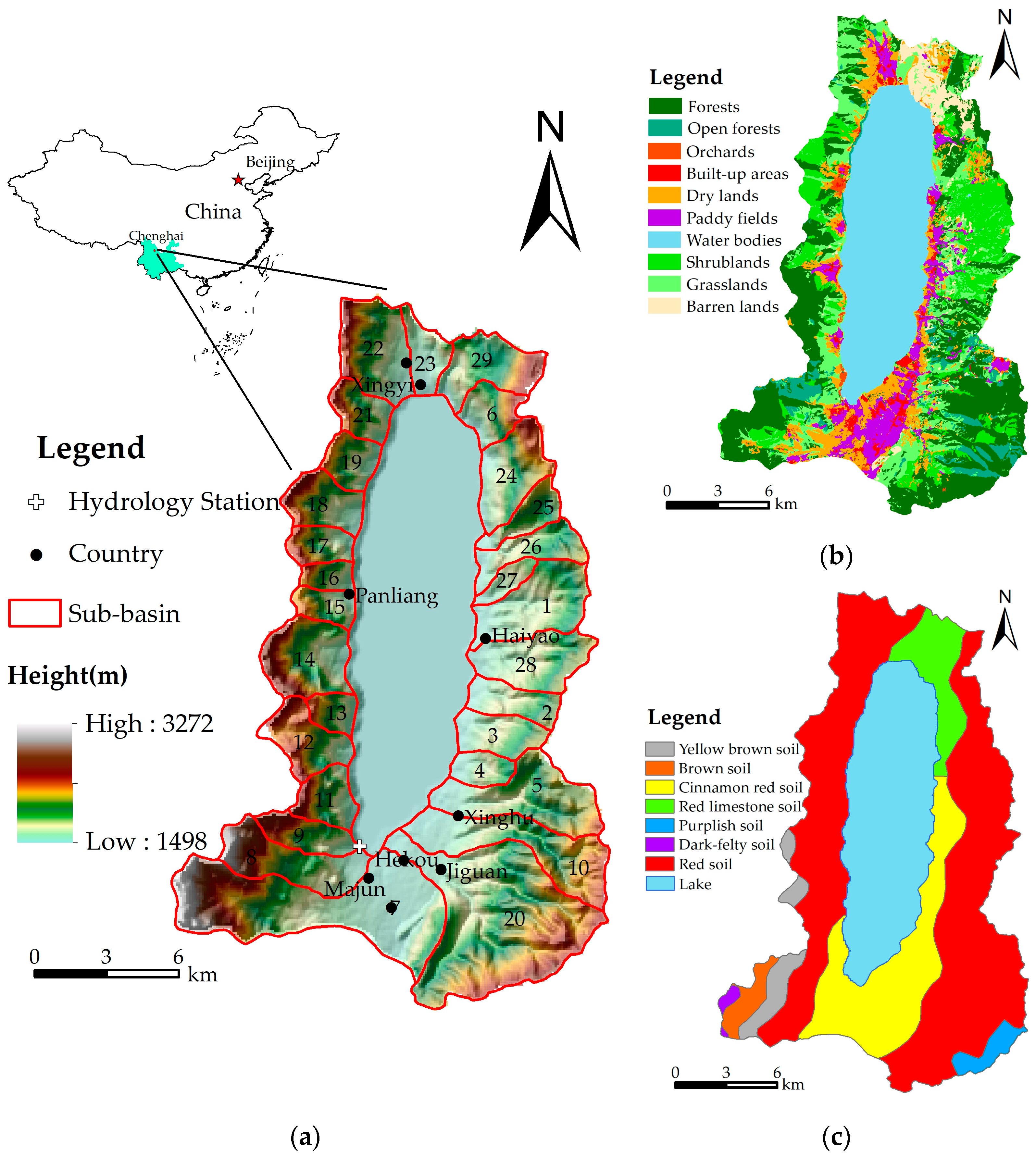
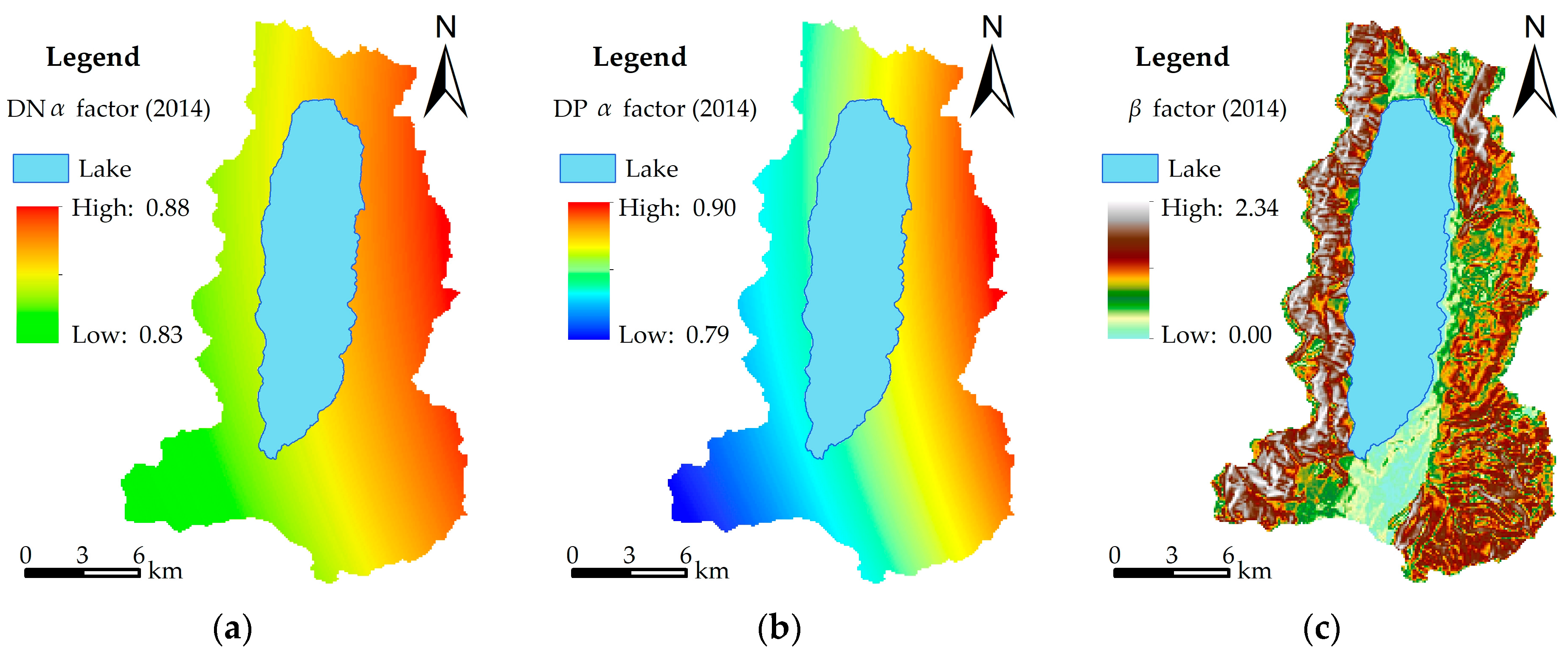
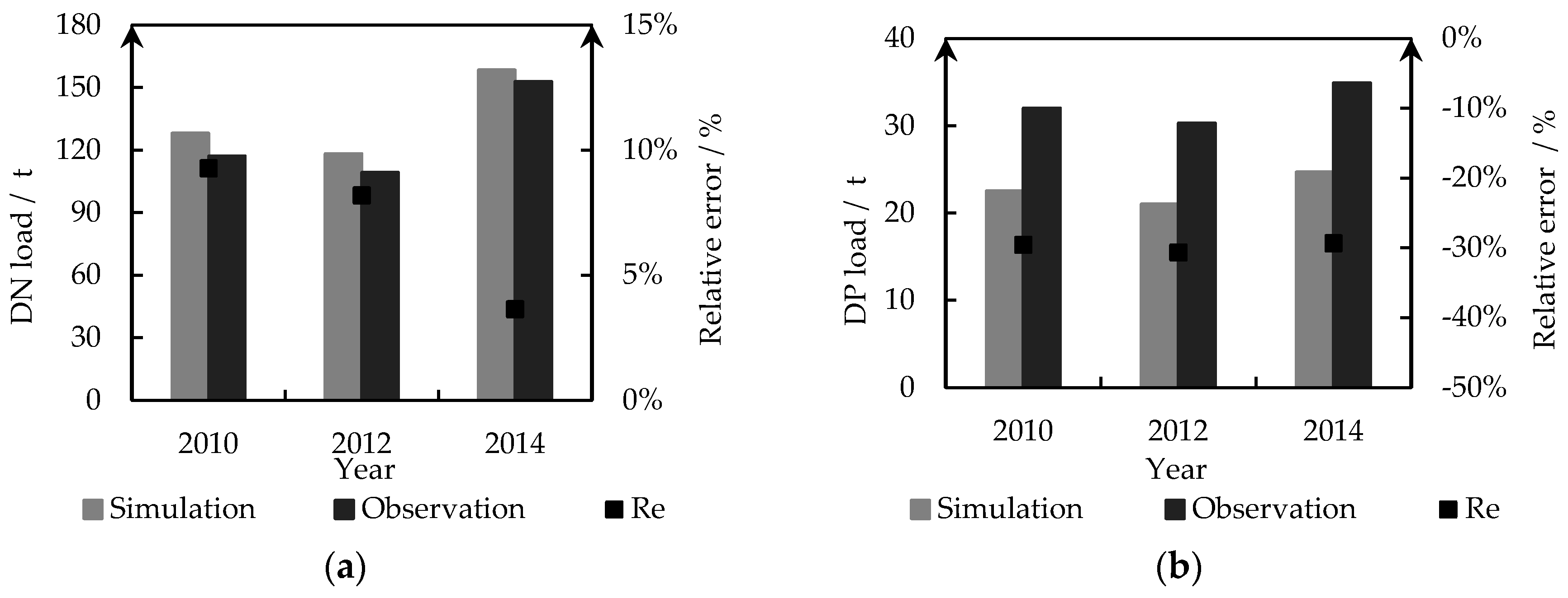
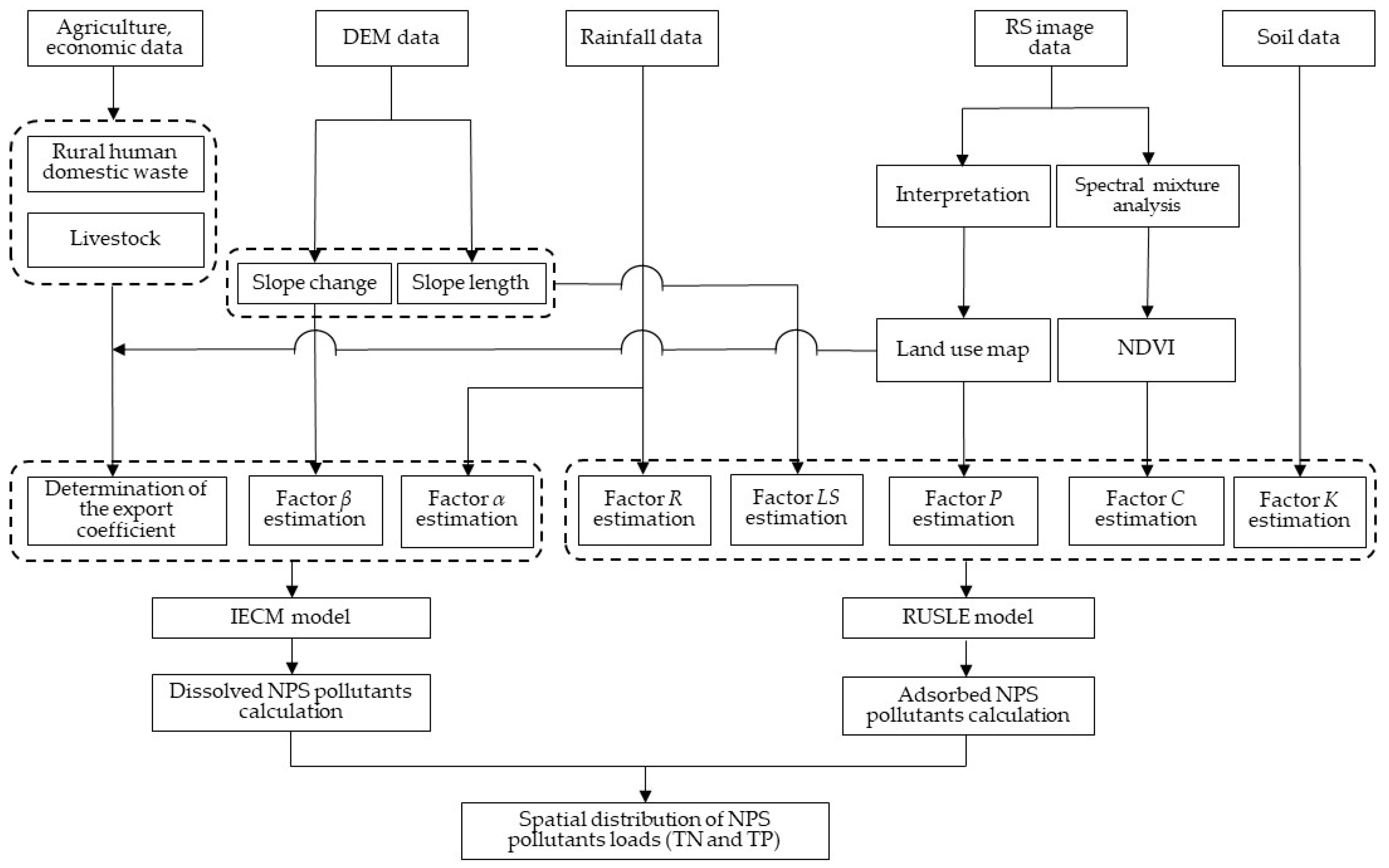
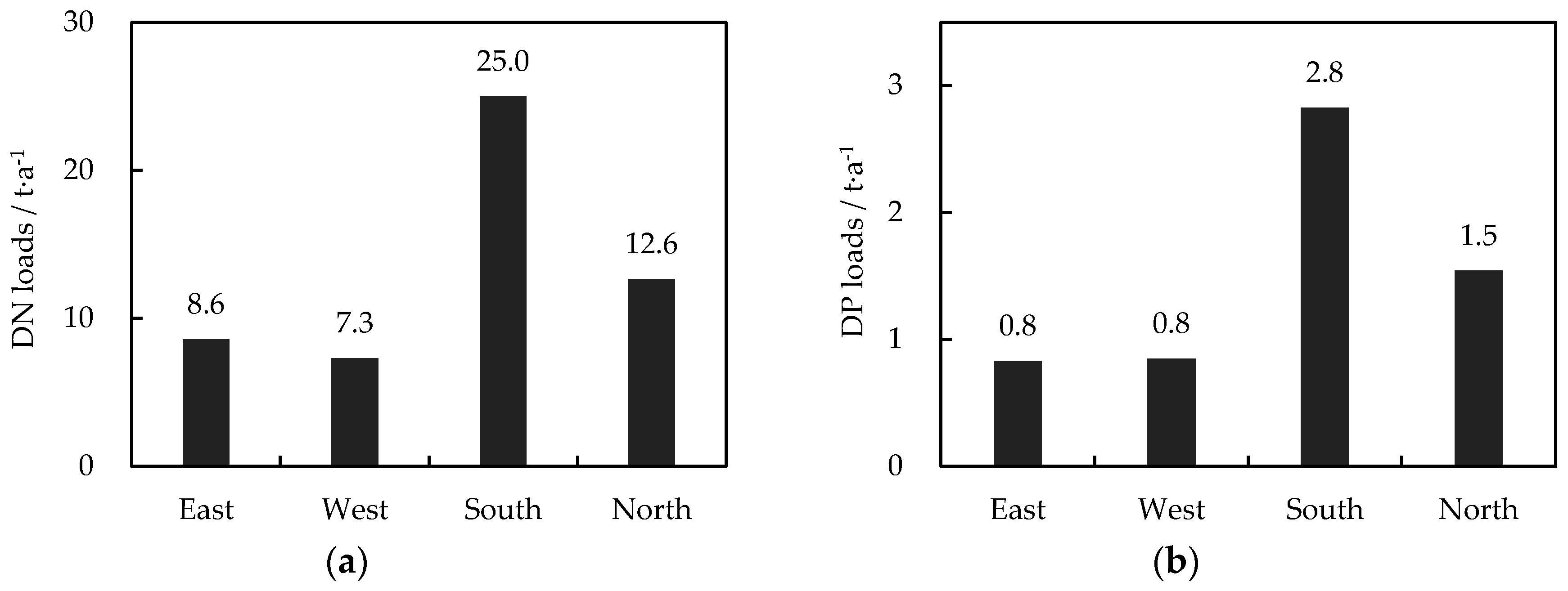
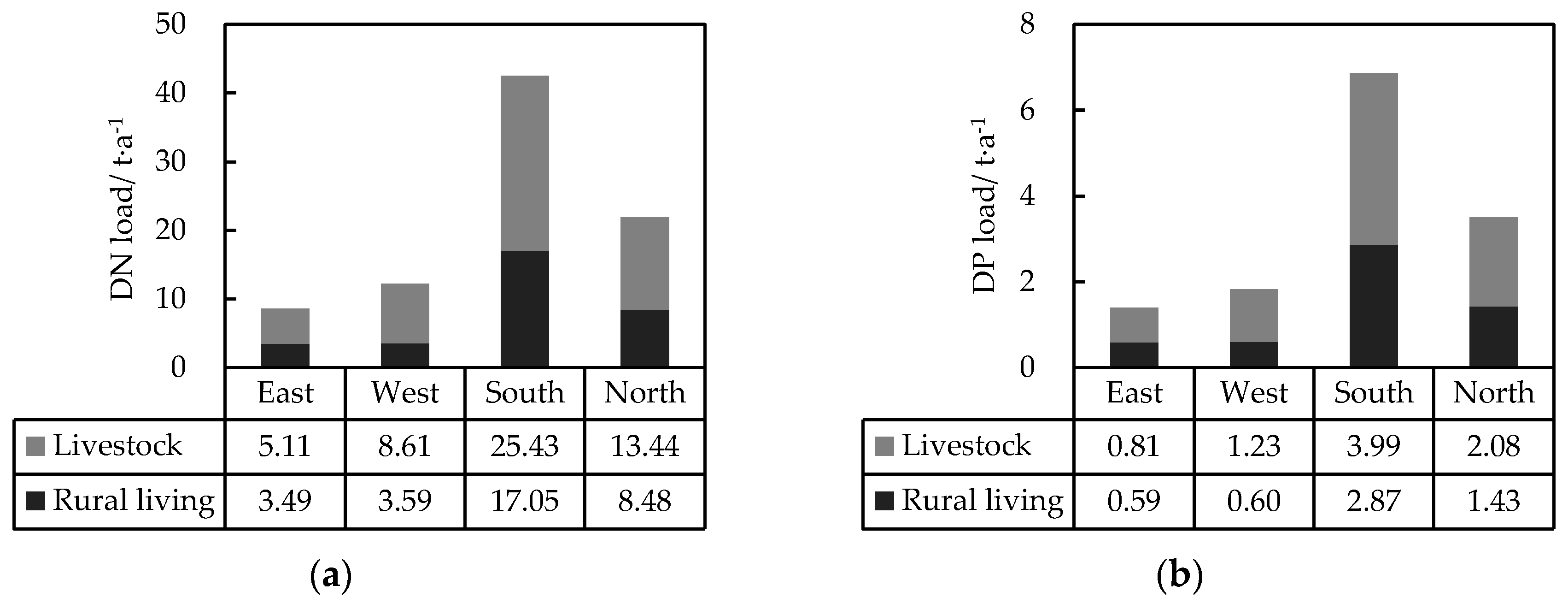
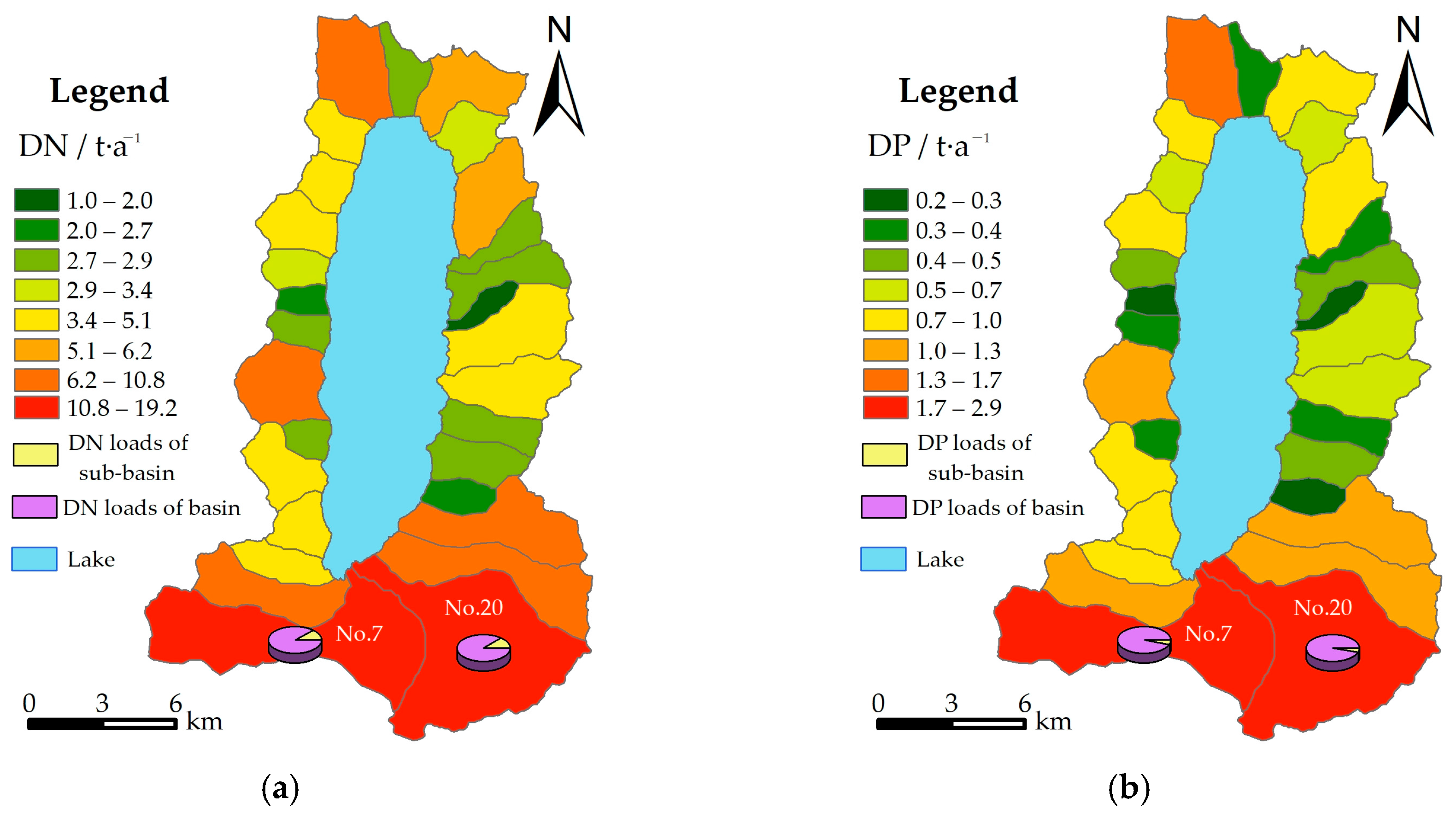
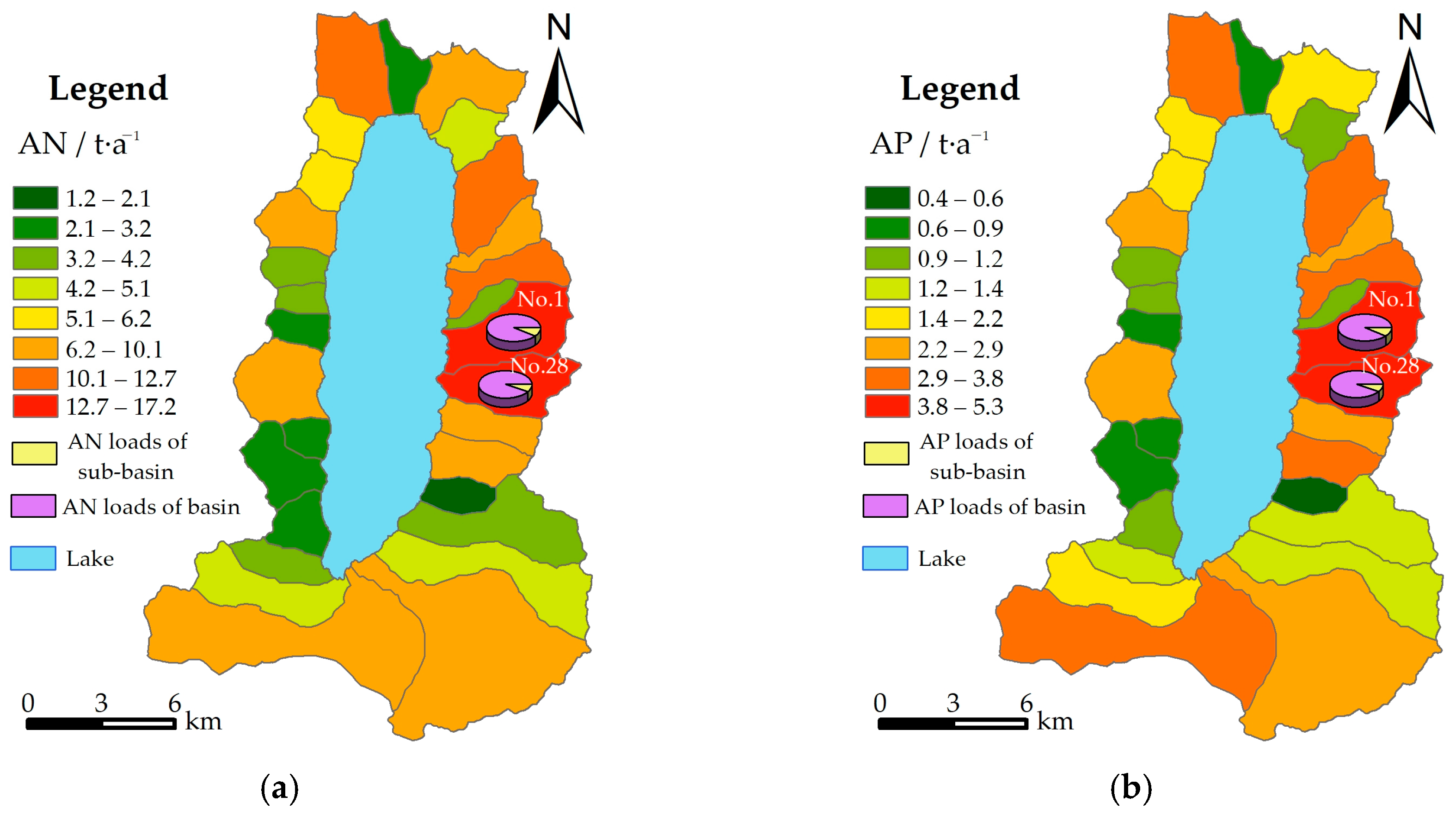
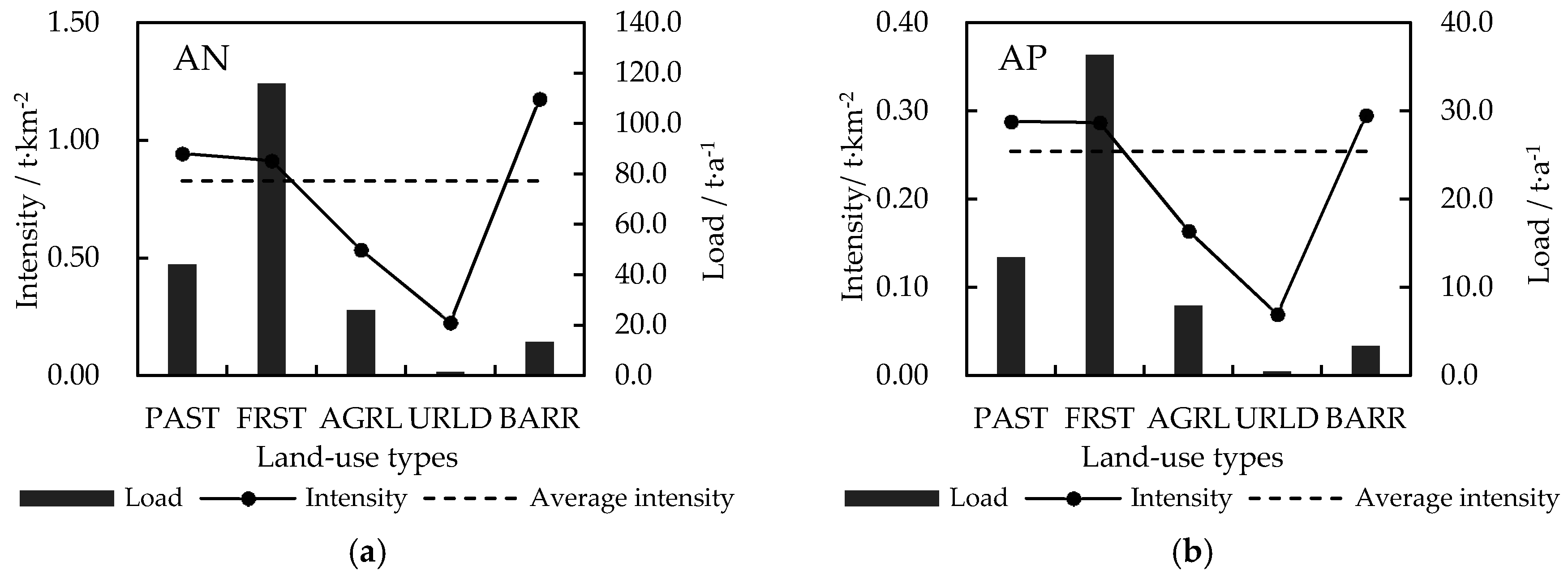
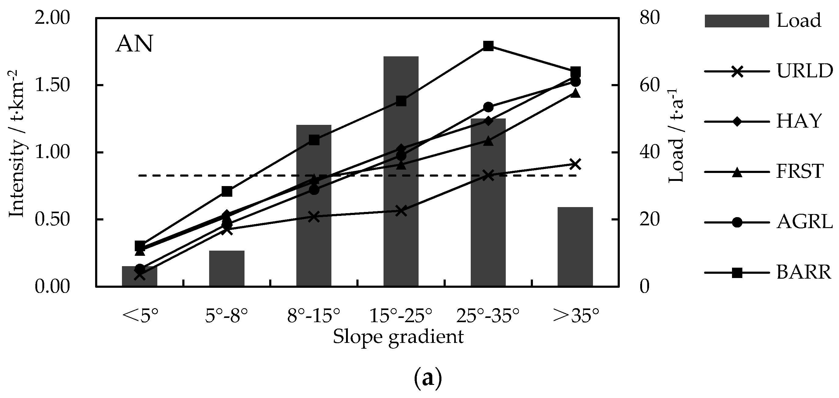
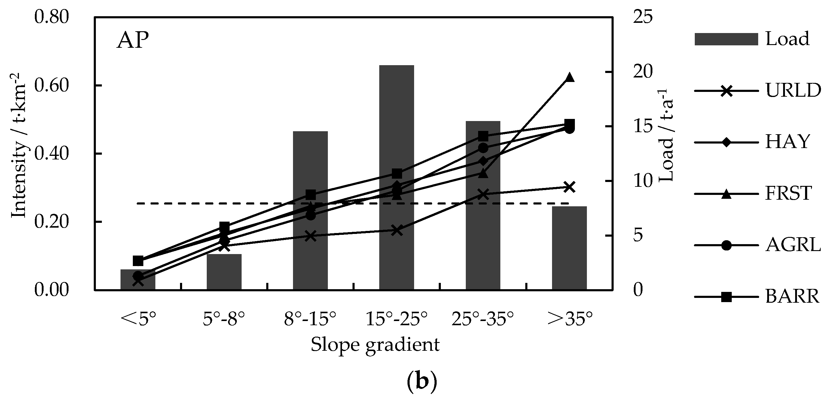
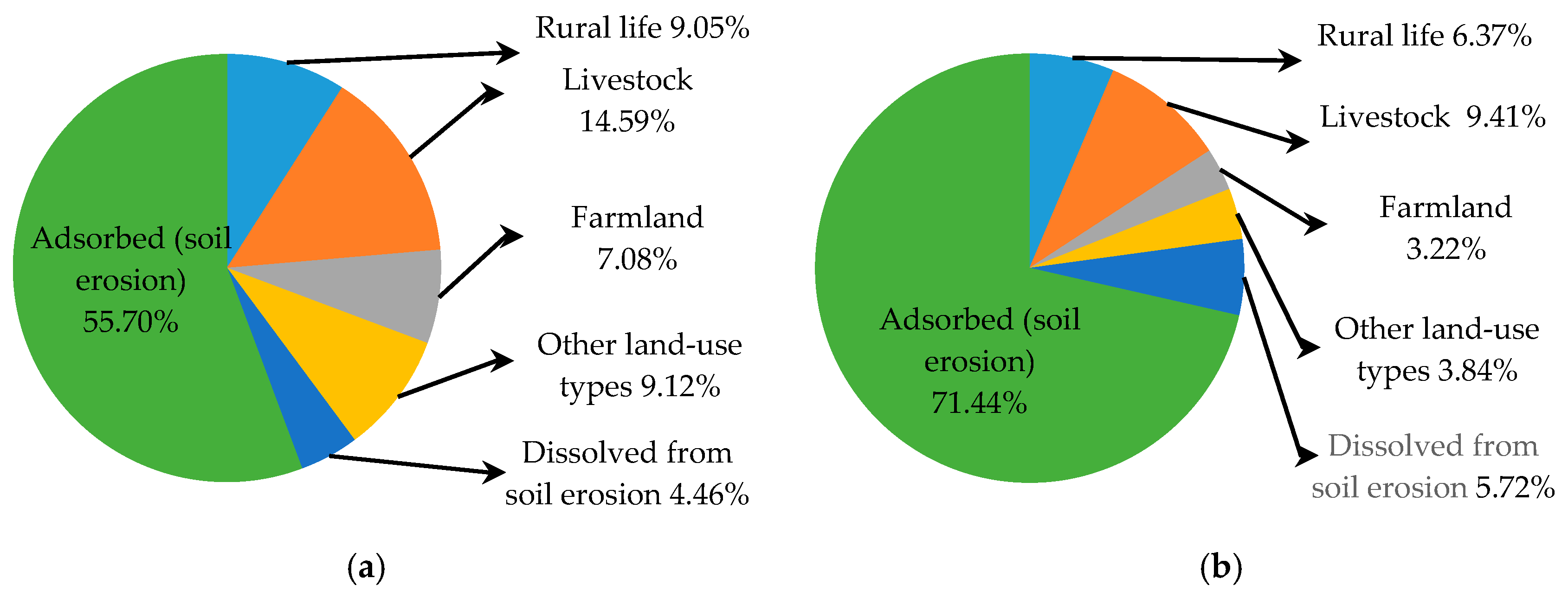
Table 1.
Yearly export coefficients for the different land-use types reported by various studies.
| Study Area | Pollutant | Export Coefficients in t (km2 a)−1 | Reference | ||||
|---|---|---|---|---|---|---|---|
| AGRL | FRST | PAST | URLD | BARR | |||
| Upper reach of the Yangtze River | DN | 4.51 | 1.28 | 0.06 | 1.12 | 1.49 | [55] |
| Upper reach of the Yangtze River | DN | 2.90 | 0.24 | 1.00 | 1.10 | 1.49 | [56] |
| DP | 0.09 | 0.02 | 0.02 | 0.02 | 0.05 | ||
| Luxian county, Sichuan Province | DN | 2.90 | 0.36 | 0.60 | 1.12 | 1.49 | [57] |
| DP | 0.60 | 0.06 | 0.20 | 0.02 | 0.05 | ||
| Dianchi watershed, Yunnan Province | DN | 2.32 | 0.25 | 0.60 | 1.30 | 1.34 | [58] |
| DP | 0.16 | 0.02 | 0.17 | 0.05 | 0.05 | ||
| Bailu River, Sichuan Province | DN | 2.88 | 0.36 | 0.60 | 1.33 | 1.15 | [59] |
| DP | 0.59 | 0.06 | 0.12 | 0.28 | 1.06 | ||
| Mangxi River, Sichuan Province | DN | 1.70 | 0.28 | NA | NA | 1.10 | [60] |
| Yunlong Reservoir of Kunming City, Yunnan Province | DN | 3.20 | 0.28 | 0.64 | NA | NA | [61] |
| DP | 0.23 | 0.02 | 0.04 | NA | NA | ||
| Upper reach of the Yangtze River | DN | 2.90 | 0.24 | 1.00 | 1.10 | 1.49 | [62] |
| DP | 0.09 | 0.02 | 0.02 | 0.02 | 0.05 | ||
| Chenghai | DN | 2.70 | 0.41 | 0.72 | 1.18 | 1.36 | This study |
| DP | 0.29 | 0.03 | 0.09 | 0.08 | 0.21 | ||
Note: NA, no data.
Table 2.
Export coefficients for the studied DN and DP pollutant sources.
| Pollution Sources | DN | DP | |
|---|---|---|---|
| Rural population [63] in kg (ca a)−1 | Domestic sewage | 0.22 | 0.03 |
| Domestic waste | 0.64 | 0.26 | |
| Fecal discharge | 1.28 | 0.22 | |
| Livestock [64] in kg (ca a)−1 | Cattle | 6.68 | 0.55 |
| Pigs | 0.80 | 0.20 | |
| Goats | 1.13 | 0.40 | |
| Poultry | 0.01 | 0.01 | |
| Land use in t (km2 a)−1 | Farmlands | 2.70 | 0.29 |
| Woodlands | 0.41 | 0.03 | |
| Grasslands | 0.72 | 0.09 | |
| Built-up areas | 1.18 | 0.08 | |
| Barren lands | 1.36 | 0.21 | |
Table 3.
DN and DP loads discharged into Lake Chenghai from the different land-use types.
| Land-Use Type | DN | DP | ||||
|---|---|---|---|---|---|---|
| Intensity in t (km2 a)−1 | Load in t a−1 | Load Fraction in % | Intensity in t (km2 a)−1 | Load in t a−1 | Load Fraction in % | |
| Grasslands | 0.22 | 10.2 | 17.49 | 0.03 | 1.3 | 21.53 |
| Shrublands | 0.13 | 4.8 | 8.20 | 0.01 | 0.4 | 5.87 |
| Dry lands | 0.62 | 17.6 | 30.19 | 0.07 | 1.9 | 31.49 |
| Built-up areas | 0.17 | 1.2 | 2.01 | 0.01 | 0.1 | 1.33 |
| Barren lands | 0.30 | 3.3 | 5.72 | 0.05 | 0.5 | 8.58 |
| Paddy fields | 0.39 | 7.9 | 13.49 | 0.04 | 0.9 | 14.06 |
| Forests | 0.13 | 10.2 | 17.42 | 0.01 | 0.8 | 12.41 |
| Open forests | 0.14 | 1.7 | 2.97 | 0.01 | 0.1 | 2.10 |
| Orchards | 0.66 | 1.5 | 2.51 | 0.07 | 0.2 | 2.61 |
Table 4.
Loads and contribution percentages of DN and DP from the different portions of the Lake Chenghai watershed.
Table 4.
Loads and contribution percentages of DN and DP from the different portions of the Lake Chenghai watershed.
| Region | DN | DP | ||
|---|---|---|---|---|
| Load in t a−1 | Percentage in % | Load in t a−1 | Percentage in % | |
| South | 78.5 | 49.51 | 12.4 | 50.16 |
| North | 37.1 | 23.40 | 5.9 | 24.01 |
| East | 21.6 | 13.63 | 3.2 | 13.04 |
| West | 21.3 | 13.46 | 3.2 | 12.79 |
Table 5.
Loads and contribution ratios of AN and AP from different regions.
| Region | AN | AP | ||
|---|---|---|---|---|
| Load in t a−1 | Percentage in % | Load in t a−1 | Percentage in % | |
| Eastern | 79.0 | 39.38 | 24.1 | 39.20 |
| Western | 27.7 | 13.78 | 8.6 | 13.99 |
| Southern | 44.7 | 22.27 | 15.5 | 25.12 |
| Northern | 49.3 | 24.57 | 13.4 | 21.69 |
Table 6.
NPS pollution control regional division.
| Name | Regional Division | Area | Causes of Pollution | |
|---|---|---|---|---|
| km2 | % | |||
| Conservation region | The lake and its 100-m buffer zone at its maximum operating water level of 1501 m | 80.56 | 25.31 | The rural population and livestock |
| Control region | The region from the buffer zone to the foot of the mountains, mainly including the areas where URLD and AGRL are relatively concentrated | 80.59 | 25.32 | The rural population, livestock and agriculture |
| Repair region | Mountainous areas, excluding the conservation region and the control region | 161.92 | 50.91 | Soil erosion |
Table 7.
Typical scenarios.
| Scenario | Livestock and the Rural Population | Farmland and Fertilizer Loss | Soil Erosion |
|---|---|---|---|
| S0 | Present levels | Present levels | Present levels |
| S1 | P1 | Present levels | Present levels |
| S2 | P2 | Present levels | Present levels |
| S3 | Present levels | P1 | Present levels |
| S4 | Present levels | P2 | Present levels |
| S5 | P2 | P1 | Present levels |
| S6 | P2 | P2 | Present levels |
| S7 | P2 | P2 | P1 |
| S8 | P2 | P2 | P2 |
© 2017 by the authors. Licensee MDPI, Basel, Switzerland. This article is an open access article distributed under the terms and conditions of the Creative Commons Attribution (CC BY) license (http://creativecommons.org/licenses/by/4.0/).
Share and Cite
MDPI and ACS Style
Chen, X.; Liu, X.; Peng, W.; Dong, F.; Huang, Z.; Wang, R. Non-Point Source Nitrogen and Phosphorus Assessment and Management Plan with an Improved Method in Data-Poor Regions. Water 2018, 10, 17. https://doi.org/10.3390/w10010017
AMA Style
Chen X, Liu X, Peng W, Dong F, Huang Z, Wang R. Non-Point Source Nitrogen and Phosphorus Assessment and Management Plan with an Improved Method in Data-Poor Regions. Water. 2018; 10(1):17. https://doi.org/10.3390/w10010017
Chicago/Turabian StyleChen, Xuekai, Xiaobo Liu, Wenqi Peng, Fei Dong, Zhihua Huang, and Ruonan Wang. 2018. "Non-Point Source Nitrogen and Phosphorus Assessment and Management Plan with an Improved Method in Data-Poor Regions" Water 10, no. 1: 17. https://doi.org/10.3390/w10010017
Note that from the first issue of 2016, this journal uses article numbers instead of page numbers. See further details here.